A Controlled Mixing Method for Stabilizing the Purity and Reducing the Waste in Gas Delivery Systems

(1)

ISSN Online: 2160-0406 ISSN Print: 2160-0392

DOI: 10.4236/aces.2019.91002 Dec. 26, 2018 11 Advances in Chemical Engineering and Science

A Controlled Mixing Method for Stabilizing the

Purity and Reducing the Waste in Gas Delivery

Systems

Junsheng Wu, Farhang Shadman

Department of Chemical and Environmental Engineering, University of Arizona, Tucson, Arizona, USA

Abstract

The variation of impurity concertation in the ultra-high purity (UHP) gases, delivered from cryogenic storage tanks and transported through long pipes, is a major problem in systems like those used in semiconductor manufacturing facilities. A method is developed for stabilizing the purity and reducing the gas consumption in these systems. This technique uses a dynamically con-trolled mixing of gases supplied by multiple cryogenic tanks. The control scheme uses software modules that simulate the processes that cause purity variation in both the cryogenic tanks and the transport lines. These processes include vaporization and supply in tanks, various modes of transport in deli-very pipes, and the adsorption and desorption on surfaces. The method also includes and corrects for variations caused by transience in gas usage rate as well as ambient conditions.

Keywords

High-Purity Gases, Cryogenic, Impurity Drift, Moisture

1. Introduction

Ultra-high-purity (UHP) gases are widely used in semiconductor fabrication plants (fabs), both as reactants in some processes like deposition and etching [1] [2], and as inert gases for purging various parts of the system. For example, UHP nitrogen is used in very large quantities in semiconductor fabs as diluent and purge medium. The UHP gases are typically delivered through pipes from gas storage facilities outside the fab to the point of use (POU). UHP gases, such as nitrogen, are usually stored in the cryogenic tanks where gas is produced by controlled vaporization of the stored liquid and transported through delivery How to cite this paper: Wu, J.S. and

Shadman, F. (2019) A Controlled Mixing Method for Stabilizing the Purity and Re-ducing the Waste in Gas Delivery Systems. Advances in Chemical Engineering and Science, 9, 11-26.

https://doi.org/10.4236/aces.2019.91002

Received: November 27, 2018 Accepted: December 23, 2018 Published: December 26, 2018

http://creativecommons.org/licenses/by/4.0/

(2)

DOI: 10.4236/aces.2019.91002 12 Advances in Chemical Engineering and Science pipes to the fab. Most semiconductor processes are very sensitive to impurities and require a well-controlled quality [3] [4]. Failure to maintain a stable purity level at the (POU) can lower the performance of process tools and even slow or shut down the processing line [5].

Moisture, selected as the model impurity species in this study, is one of the most common impurities. While affecting many fabrication processes even at the parts per billion (ppb) levels, it is also one of the most challenging impurities to remove and control due to its strong adsorption on the surfaces of transport line, components, and reactors [3] [6] [7]. Additionally, when gases are supplied from cryogenic sources, there is usually some drift and variation in the moisture level at the POU due to two major factors [8]:

1) Source drift: This is caused by the build-up of moisture in the cryogenic tanks due to the selective retention of moisture in the liquid phase during vapo-rization. As impurity level goes up with time and gas usage, and the gas purity can no longer satisfy the process requirements (usually after 70% - 80% of a tank is used), the remaining content is rejected and wasted, causing financial and en-vironmental losses.

2) Temperature-induced variations: This is caused by adsorption (capture) and desorption (release) of moisture on the surfaces of delivery pipes and flow-control devices. The delivery pipes in most fabs are long and therefore a major sink for moisture adsorption. Moreover, these pipes, running from the storage area to the POU are usually in the open environment. Therefore, am-bient temperature variations would have a large effect on the moisture adsorp-tion and desorpadsorp-tion, leading to drifts and spikes in impurity at the POU.

Single tank systems are widely used as cryogenic sources for many gases in industry today. However, this configuration results in impurity drift due to se-lective retention and accumulation of impurities in one phase during vaporiza-tion. For example, moisture is selectively retained in the liquid phase of most in-ert and process gas tanks, resulting in impurity drift upward, as liquid is vapo-rized and gas is withdrawn from the cryogenic tank. The drift necessitates shut-ting down the supply when the impurity level reaches the highest acceptable lev-el. At this time, the partially used tank needs to be returned to the supplier, often with large amount of gas remaining unused in the tank. This increases the cost and the negative environmental impact of the operation due to the partial usage of tank content.

In recent years, some modifications have been introduced in cryogenic tank design to reduce the effect of source drift [9]. These changes increase the cost and the complications of supply tanks significantly. However, there has been no systematic study of disturbances caused by pipelines or developments of tech-niques to mitigate them. Purifiers can be used to remove moisture at the POU

(3)

DOI: 10.4236/aces.2019.91002 13 Advances in Chemical Engineering and Science the POU [10]. The objective of the current work has been to develop a method for mitigating the effects of the variations in impurity levels, caused by the above two factors and assuring a stable and well-controlled purity level at the POU.

2. Method of Approach

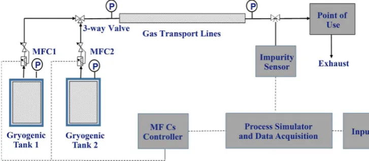
The proposed concept and the associated system in this study are schematically shown in Figure 1. The system, chosen to illustrate the method, consists of two cryogenic tanks, two mass flow controllers (MFC), a gas delivery system, a real-time sensor for on-line measurement of impurities, and the auxiliary elec-tronics for running the process simulator, data acquisition, and MFCs program-ing and control. The flow streams from the two tanks are controlled by two MFCs, then mixed and transported to the POU through a transport pipeline. The impurity level at the POU is monitored by an online sensor. The process simulator provides input to the MFC controller unit that adjusts the flow out of each MFC. Overall, the set-up provides a dynamic flow-mixing scheme run by the output from the process simulator. The system properties, operating condi-tions and purity requirements are all inputs to the process simulator. The details of the process simulator and its functions are described in the following two sec-tions: first one for cancelling the drift in the cryogenic tanks and the second one for mitigating the effects of the pipeline temperature variations.

2.1. Multiple Tanks to Resolve the Source Drift Problem

As pointed out in the Introduction section, the single-tank configuration results in impurity drift due to the accumulation of impurities like moisture in the liq-uid phase during vaporization. This leads to partial usage of tank content and wasting of gas. To resolve this drift issue, a dual tank system is proposed, where flow rates from two tanks are varied and mixed so that a stable and well-controlled purity level is obtained.

[image:3.595.158.522.546.705.2]

Assuming that gas and liquid in the tank are in equilibrium, the following eq-uations determine the operation of tank 1:

(4)

DOI: 10.4236/aces.2019.91002 14 Advances in Chemical Engineering and Science 1 1 1

g l t

V +V =V (1)

1 1 1 1 1

t g l l

C V +C V =M ₍₂₎

1 1

d

dM_t C Qt

− = ₍₃₎

1 1 g l

Y =Y H₍₄₎

1 1 d d d d g l V V _Q

t α t

− = + _{, (5)}

where Vt1, Vg1, and Vl1 are the total tank volume, the gas phase volume, and

the liquid phase volume in the tank, respectively. Ct1 and Cl1 are the impurity

concentrations in the vapor and liquid phases in the tank, M1 is the total amount

of impurity in the tank, Q is the withdrawn flow rate, Yg1 and Yl1 are the mole

fractions of impurity in the vapor and the liquid phases, H is Henry’s law constant, and α is the ratio of liquid to vapor densities. Equations (2) and (3) together are the mass balance for the impurity in the tank; Equation (4) shows the liquid-vapor equilibrium for the impurity, and Equation (5) is the overall balance for gaseous content. Solving these five equations simultaneously gives:

1 d

d g

V Q

t =α (6)

(

)

1

1 1 1 d d t t l

Q H C

C

t αV

−

= _{. (7)}

The total flow rate, Q, which is the sum of the flow rates from the tanks is given by the process demand at the POU. The flow rate from the first tank, Q1,

as a fraction of Q, is given by:

1

Q bQ= _{. (8)}

Equations (6) and (7) can be modified as

1 d

d g

V _bQ

t = α (9)

(

)

1

1 1 1 d d t t l bQ H C C

t αV

−

= _{. (10)}

Similarly, the equations in tank 2 are

(

)

2

d 1

d g

V b Q

t α

−

= ₍₁₁₎

(

) (

)

2

2 2 1 1 d d t t l b Q H C C

t αV

− −

= _{. (12)}

The impurity concentration in the mixed flow from two tanks is

(

)

1 1 2

t t t

C =bC + −b C _{. (13)}

Given any desired C tt

( )

function, the mixing function, b t

( )

, is given by:

2 1 2 t t t t C C b C C − =

(5)

DOI: 10.4236/aces.2019.91002 15 Advances in Chemical Engineering and Science

2.2. Programmed Mixing to Mitigate the Temperature-Induced

Variations

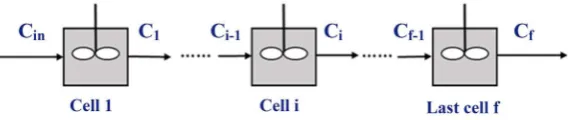
The analysis of the processes taking place in the pipeline is through solving the conservation equations of transport and reactions in the pipe. However, applica-tion of the convenapplica-tional numerical approach in this particular case is compli-cated since the inlet concentration is not known; the known boundary condition is the outlet and not the inlet concentration. The proposed solution to this nu-merical issue is the use of an equivalent system model consisting of a series of well-mixed cell, shown in Figure 2, where the number of cells is selected to represent the extent of dispersion in the pipe. This modeling approach is widely used in the analysis of non-ideal tubular reactors [11].

The mass balance for impurity in the gas phase for the first cell is given by

(

)

1

1 1 1 0 1 d_d

in S d s a s V C

C C k C k C S C

Q  Q t

− + _ − − _= ₍₁₅₎

The mass balance for any intermediate cell i in the chain is

(

)

-1 0 d_di

i i S d si a i si V C

C C k C k C S C

Q  Q t

− + _ − − _= ₍₁₆₎

and the corresponding equation for the last cell is

(

)

1 0

d d

f

f f d sf a f sf

C

S V

C C k C k C S C

Q Q t

− − +  − − = (17)

The mass balance equations for the impurity adsorbed on the pipe surface are

(

)

1

1 0 1 1 d_ds

a s d s C

k C S C k C t

− − = ₍₁₈₎

(

0

)

d_dsi

a i si d si C k C S C k C

t

− − = _{for any cell}_{i in the chain (19)}

(

0

)

d d

sf

a f sf d sf

C

k C S C k C

t

− − = _{, (20)}

where Cin and C1 are the inlet and the outlet impurity concentrations of the

first cell; Ci−1 and Ci are the inlet and the outlet impurity concentrations of

cell i; similarly, Cf−1 and Cf are the inlet and outlet impurity concentrations

of the last cell. Cs1, Csi, and Csf are the adsorbed concentrations in these

cells; ka is the adsorption rate constant, kd is the desorption rate constant,

and S0 is the surface site density in each cell; S is the surface area of each cell, V

[image:5.595.233.524.646.706.2]

is the cell volume, and Q is the total volumetric flow rate. The initial conditions of Equations (15) to (20) are

(6)

DOI: 10.4236/aces.2019.91002 16 Advances in Chemical Engineering and Science at t=0,Cs1=Csi =Csf =Cs0 (21) at t=0,Cin =C C1= i−1=C Ci= f−1=Cf =C0, (22)

where Cs0 is the initial adsorbed concentration, C0 is the initial gas phase

concentration, and Cs0 is the adsorbed concentration in equilibrium with C0.

The adsorption rate constant, ka, and the desorption rate constant, kd, are

functions of temperature, given by

e aa

E RT a

k −

∝ (23)

e ad

E RT d

k −

∝ , (24) where Ea and Ed are the activation energies for adsorption and desorption,

R is gas constant, and Ta is ambient temperature in the pipe.

When the mixed flow enters the pipe, its temperature rises from tank temper-ature, Tt, to the pipe temperature which is assumed to be the ambient

tempera-ture, Ta. Therefore, the mixed concentration, Ct, is related to the inlet

concen-tration of cell 1, Cin, by

t

in t

a

T

C C

T

= _{, (25)}

and the change in the outlet concentration of the last cell, Cf , with temperature

is given by

0 0 f

a

T

C C

T

= _{, (26)}

where T0 is the initial temperature in the pipe.

For a given desired Cf, the function b t

( )

, which is the ratio of flow rate

from tank 1 to the total flow rate, is determined by the simultaneous solution to the above equations.

3. Results and Discussion

3.1. Two-Tank Configuration for Canceling the Impurity Drift

Nitrogen and moisture are selected as the model main gas and impurity, re-spectively in this example. However, the methodology and the process simu-lator tool are not limited to these two compounds and can be applied to other gases as well. In this example, two tanks are used simultaneously as the cryo-genic source for nitrogen. Initially, tank 1 is a partially used and tank 2 is a new full tank. Since the typical gas usage in semiconductor processing tools is transient and periodic, a cyclic flow rate is used to represent the total gas sup-plied by the system.

In general, the present analysis can be used to determine the mixing func-tion b t

( )

needed for obtaining any desired impurity concentration in the mixed flow from the cryogenic tanks, C tt

( )

. In this example, the desired

concentration, C tt

( )

, is assumed to be constant. The parameters used in this

(7)

[image:7.595.210.540.89.312.2]

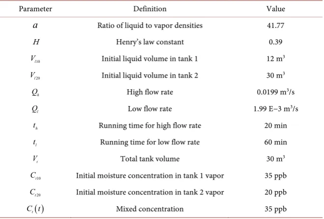
Table 1. Parameters in two-tank model study.

Parameter Definition Value

a Ratio of liquid to vapor densities 41.77

H Henry’s law constant 0.39

10

l

V Initial liquid volume in tank 1 12 m3

20

l

h

Q High flow rate 0.0199 m3_/s

l

Q Low flow rate 1.99 E−3 m3_/s

h

t Running time for high flow rate 20 min

l

t Running time for low flow rate 60 min

t

V Total tank volume 30 m3

10

t

C Initial moisture concentration in tank 1 vapor 35 ppb

20

t

( )

t

C t Mixed concentration 35 ppb

from experimental data presented in previous study [10]. It is assumed that the flow rate needed at the POU alternates between a low value and a high value at regular intervals. This kind of variation is typical for most semicon-ductor fabrication applications and tools. Using the analysis method of Sec-tion 2.1, the mixing funcSec-tion, b t

( )

, that gives a constant mixed concentration

( )

35 ppb

t

C t = _{, is determined; the results are shown in}_{Figure 3}_.

The mixing function profile shows that initially b t

( )

=1_{, indicating that the}

mixed flow is fully supplied from tank 1. As time goes on, b t

( )

decreases be-cause the moisture level in tank 1 increases and more flow from tank 2 is re-quired to compensate for this increase. After about 44 hours, b t

( )

is nearly zero, indicating that the mixed flow is almost provided from tank 2. At this time, moisture level in tank 1 is too high and the desired mixed concentration cannot be obtained by mixing the flow from these two tanks. Therefore, a tank change is needed at this time to replace the exhausted tank 1 with a new tank.

Figure 4 shows liquid volume in two tanks during this 44-hour cycle before tank replacement. At the end of this cycle, the liquid volume in tank 2 decreases from 30 m3_{to 12.1 m}3_{, which is almost the same volume as the initial liquid}

vo-lume (12 m3_{) in tank 1. The liquid volume in tank 1 goes from 12 m}3_{to 2.4 m}3

after 44 hours. The 44-hour cycle represents the lifetime of tank 1 before replac-ing it with a new tank. At this time, tank 2 is in conditions similar to that of tank 1 at the beginning of the cycle. Therefore, a new cycle starts and repeats the same changes. After each cycle, the tank which runs out of liquid nitrogen will be taken out for recharge or replacement.

(8)

[image:8.595.222.531.77.255.2]

[image:8.595.230.520.290.469.2]

Figure 3.Temporal profile of the mixing function, b t

( )

.

Figure 4.Temporal profiles of the liquid content of the two tanks.

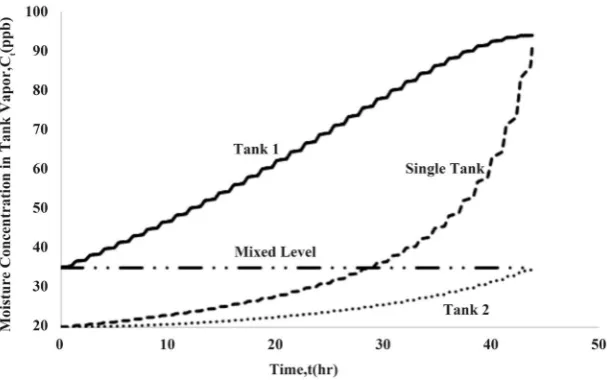
[image:8.595.222.526.505.695.2]

(9)

DOI: 10.4236/aces.2019.91002 19 Advances in Chemical Engineering and Science time; after around 28 hours, the moisture level exceeds 35 ppb. However, using the proposed controlled mixing with the appropriate mixing function, b t

( )

=1_,

a stream with constant concentration of 35 ppb is obtained and maintained for the entire cycle time. Moreover, the results show that the two-tank configuration with the proposed mixing technique results in 92% usage of the liquid nitrogen in each tank compared with less than 80% usage of liquid nitrogen in a conven-tional single-tank system.

3.2. Application of the Proposed Scheme to Cancel the Combined

Effects of Tank Drift and Pipe Temperature Variations

In this example, a more complete system is analyzed, where the delivery tanks are followed by a pipeline that takes the gas from the tanks to the POU. There-fore, the transport processes, the adsorption and desorption effects, and the temperature changes in the ambient around the pipe all contribute to the impur-ity variations at the POU. For illustration, a desired constant moisture level of 40 ppb is assumed at the POU, which is the pipe outlet in this case. A cyclic flow rate between a high value Qh and a low value Ql is used to represent the POU

re-quirement. In one cycle, Qh lasts 20 minutes, and Ql lasts 60 minutes. The

cyc-lic ambient temperature (diurnal effect) is assumed to follow:

[ ]

(

)

[ ]

π

298 15sin hr 12 K

12 a

T = + _ t + _

  . (27)

The initial moisture concentration C0 is 7.79E−6 mol/m3; therefore, the

de-sired concentration at POU is:

(

)

[ ]

(

)

[ ]

6 3 298 K

7.79 mol m

π

15sin hr 12 K

12 f

C E

t

− _ _

= _ _ ∗

 ₊ 

 

 

(28)

The mixing function b t

( )

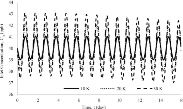
is calculated in two steps. In the first step, the inlet concentration, Cin, is determined using the mixing cells model described in

Sec-tion 2.2. The parameters of the system used in this example are listed in Table 2. In the first step, the pipe inlet concentration, Cin, is calculated from the

mix-ing cells model of Section 2.2. Cin starts as C0 and then changes due to

tem-perature variations, going down as temtem-perature goes up. The comparison of re-sults for 3 and 4 tanks in Figure 6 shows that there is not a significant difference in the final results between these two cases.

In the second step, the procedure described in Section 2.1 is used to find

( )

b t from Cin, calculated in step 1. Due to the presence of the pipeline, the

system configuration in this case is different from that of example in Section 3.1; therefore, the resulting mixing function, b t

( )

, will also be different.

(10)

[image:10.595.207.541.98.480.2]

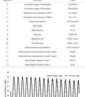
Table 2. Parameters in combination of models.

Parameter Definition Value

a

E Activation energy of adsorption 5 kcal/mol

d

E Activation energy of desorption 30 kcal/mol

0

a

k Adsorption rate constant at 298 K 5 m3_/mol·s

0

d

k Desorption rate constant at 298 K 5E−5 1/s

0

S Surface site density 1.5E−8 mol/m2

L Pipe length 100 m

d Pipe diameter 0.1 m

P Pressure 4.83E5 Pa

h

Q High flow rate 9.93E−3 m3_/s

l

Q Low flow rate 9.93E−5 m3_/s

0

C Initial moisture concentration 7.79E−6 mol/m3

10

t

20

t

10

l

V Initial liquid volume in tank 1 9.65 m3

20

l

[image:10.595.209.538.98.552.2]

Figure 6.Comparison of Cin profiles obtained by assuming 3 and 4 cells in modeling the

pipeline.

model, C tt

( )

is calculated using Equation (25). The calculated mixing function,

( )

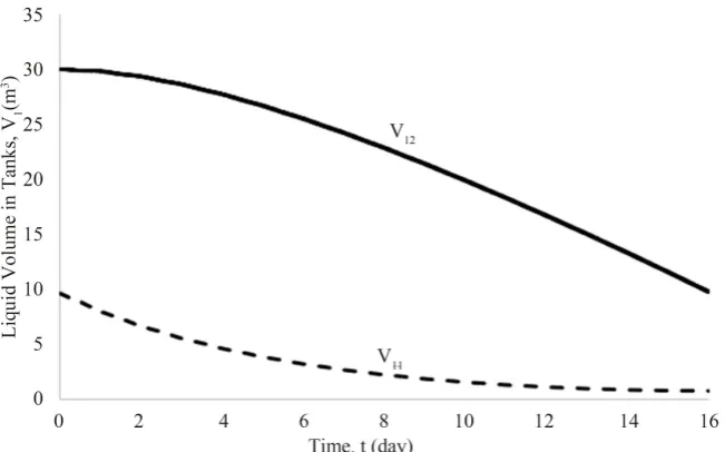
b t , and the liquid volume in tanks are shown in Figure 7 and Figure 8. The results show that at the end of 16 days, b is nearly zero. The liquid volume in tank 2 drops from 30 m3_{to 9.77 m}3_,_{which is close to the initial liquid volume}

(9.65 m3_{) in tank 1. During this time, the liquid volume in tank 1 goes from 9.65}

m3_{to 0.80 m}3_{after 16 days. Therefore, 16 days represents one cycle and the time}

(11)

[image:11.595.212.540.73.231.2]

Figure 7.Temporal profile of the mixing function, b t

( )

.

Figure 8.Temporal profiles of the liquid content of the two tanks.

the conventional single tank configuration.

3.3. Parametric Study of Temperature

An important application of the methodology developed in this study is in para-metric study for optimizing the operation of an existing system or designing a new system. Using the proposed approach, the analysis of a system over a wide range of configurations and operating conditions is relatively fast and inexpensive compared to running experiments on a physical set up. For example, to see the effect of temperature variations, three types of temperature amplitudes (10, 20, and 30 degrees centigrade) were compared, using the same temperature func-tionality given by Equation (27). The time profiles of inlet concentration, Cin,

mixing function, b t

( )

, and liquid volumes, Vl1 and Vl2 are shown in Figures

[image:11.595.213.539.263.466.2]

(12)

[image:12.595.225.523.71.248.2]

[image:12.595.223.525.287.467.2] [image:12.595.230.525.517.703.2]

Figure 9.Temporal profiles of Cin under various temperature amplitudes.

Figure 10.Temporal profiles of mixing function b t

( )

under various temperature am-plitudes.

(13)

DOI: 10.4236/aces.2019.91002 23 Advances in Chemical Engineering and Science change in the mixing function, b t

( )

.

4. Conclusions

Most semiconductor fabrication processes are very sensitive to impurities in purge and process gases. Therefore, maintaining a stable purity level in gas supply systems is of critical importance for this industry. Moisture is one of the most common and also most problematic impurities in the ultra-high-purity gases. Most UHP gases are supplied from cryogenic storage tanks and transported to the point of use (POU) by pipelines that are exposed to ambient environment. This arrangement results in variations of moisture level delivered to the POU due to two primary factors: The first is the drift due to the phase segregation of impurities during liquid vaporization in the cryogenic tanks. Moisture in most cryogenic systems segregates favorably in the liquid phase. This results in the re-tention and accumulation of moisture in the liquid phase and a gradual increase in the impurity in the gas delivered from these sources. The second factor is the variation of the impurity due to the adsorption and desorption on the surfaces of transport pipelines exposed to the varying outside temperature.

In this study, a new approach is proposed and analyzed that will cancel the variations caused by both of these two factors. In this approach, the stability and high purity at the POU are achieved through controlled mixing of gases from two cryogenic tanks. The mixing ratio is a dynamic function of time that is found through the application of a process simulator developed in this work. The simulator includes both the system geometry and configuration as well as the operating conditions and variations of external factors such as the ambient temperature. The proposed approach is expected to result in significant savings in the usage of gases. For example, compared to the conventional single-tank me-thod, which can only use less than 80% of liquid nitrogen from a liquid nitrogen tank, the proposed method increases the liquid nitrogen utilization to over 90%.

The formulation of the simulator is generally valid for most cryogenic gas supply systems. However, the continuation of this work should include applica-tion to the control of impurities in reactive gases such as moisture in ammonia, which is another key issue in the semiconductor fabs.

Acknowledgements

Financial and technical supports from Intel Corporation and the SRC Engineer-ing Research Center for Environmentally Benign Semiconductor ManufacturEngineer-ing are acknowledged.

Conflicts of Interest

The authors declare no conflicts of interest regarding the publication of this paper.

References

(14)

V.H. (2003) Contamination Control in Gas Delivery Systems for MOCVD. Journal ofCrystalGrowth, 248, 67-71. https://doi.org/10.1016/S0022-0248(02)01889-4 [2] Fine, S.M., McGuire, J.T., Choi, B.S., Bzik, T., Crofton, K.T., Melnyk, A., Perez, M.

and Sheriff, D.P. (1996) Optimizing the UHP Gas Distribution System for a Plasma Etch Tool. SolidStateTechnology, 39, 71-77.

[3] Haider, A.M. and Shadman, F. (1991) Desorption of Moisture from Stainless Steel Tubes and Alumina Filters in High Purity Gas Distribution Systems. IEEE Transac-tionsonComponents, Hybrids, andManufacturingTechnology, 14, 507-511.

https://doi.org/10.1109/33.83935

[4] Krishnan, S. and Laparra, O. (1997) Contamination Issues in Gas Delivery for Sem-iconductor Processing. IEEE TransactionsonSemiconductorManufacturing, 10, 273-278. https://doi.org/10.1109/66.572082

[5] Yao, J., Wang, H., Dittler, R., Geisert, C. and Shadman, F. (2010) Application of Pressure-Cycle Purge (PCP) in Dry-Down of Ultra-High-Purity Gas Distribution Systems. ChemicalEngineeringScience, 65, 5041-5050.

https://doi.org/10.1016/j.ces.2010.06.002

[6] Ma, C. and Verma, N. (1998) Moisture Drydown in Ultra-High-Purity Oxygen Sys-tems. JournaloftheIEST, 41, 13-15.

https://doi.org/10.17764/jiet.41.1.ym44t93qn5467505

[7] Ishihara, Y., Kurihara, S., Ishihara, S., Toda, M. and Ohmi, T. (1997) Trace Mois-ture Adsorption onto Various Stainless Steel Surface. HyomenKagaku, 18, 557-563. [8] Dittler, R., Shadman, F., Guzman, R. and Muscat, A. (2014) Reducing

Ul-tra-High-Purity (UHP) Gas Consumption by Characterization of Trace Contami-nant Kinetic and Transport Behavior in UHP Fabrication Environments, ProQuest Dissertations and Theses.

[9] Vininski, J., Yilcelen, B., Torres, R. and Houlding, V. Bulk Specialty Gas Systems for Ammonia Gas Phase Delivery vs. Liquid Phase Delivery.

http://www.mathesongas.com/electronics/technical-library

[10] Wu, J. and Shadman, F. (2018) Impurity Drift and Variations in High-Purity Gas Delivery Systems. InternationalJournal ofEngineeringandMathematical Model-ling, 2018, 1-9.

http://www.orb-academic.org/index.php/journal-of-engineering-modelling/issue/vi

ew/44

[11] Waldram, S.P. (1985) Non-Ideal Flow in Chemical Reactors. In: Waldram, S.P., Ed.,

ComprehensiveChemicalKinetics, Elsevier, Amsterdam, Vol. 23, 223-281.

(15)

Nomenclature

α

: ratio of liquid to vapor densities;

( )

b t : mixing function;

0

C : initial gas phase concentration in the pipeline, (mol/m3_);

1

C: outlet impurity concentration of the first cell, (mol/m3_);

1 f

C − : inlet impurity concentration of the last cell, (mol/m3);

f

C : outlet impurity concentration of the last cell, (mol/m3_);

1 i

C− : inlet impurity concentration of cell i, (mol/m3);

i

C: outlet impurity concentration of cell i, (mol/m3_);

in

C : inlet impurity concentration of the first cell, (mol/m3_);

1 l

C : impurity concentration of the liquid phase in tank 1, (mol/m3_);

1 s

C : adsorbed concentration in the first cell, (mol/m2_);

sf

C : adsorbed concentration in the last cell, (mol/m2_);

si

C : adsorbed concentration in cell i, (mol/m2_);

0 s

C : initial adsorbed concentration, (mol/m2_);

t

C: mixed concentration, (mol/m3_);

1 t

C : impurity concentration of the vapor phase in tank 1, (mol/m3_);

10 t

C : initial impurity concentration of the vapor phase in tank 1, (mol/m3_);

2 t

C : impurity concentration of the vapor phase in tank 2, (mol/m3_);

20 t

C : initial impurity concentration of the vapor phase in tank 2, (mol/m3_);

d: pipe diameter, (m);

a

E : activation energy for the adsorption, (kcal/mol);

d

E : activation energy for the desorption, (kcal/mol); H: Henry’s law constant;

a

k : adsorption rate constant, (m3_/mol·s);

0 a

k : adsorption rate constant at 298 K, (m3_/mol·s);

d

k : desorption rate constant, (1/s);

0 d

k : desorption rate constant at 298 K, (1/s); L: pipe length, (m);

1

M : total amount of impurity in tank 1, (mol); P: pressure, (Pa);

Q: volumetric flow rate, (m3_/s);

1

Q: flow rate from tank 1, (m3_/s);

h

Q : high flow rate, (m3_/s);

l

Q: low flow rate, (m3_/s);

R: gas constant, (J/mol·K); S: surface area of each cell, (m2_);

0

S : surface site density in each cell, (mol/m2_);

h

t : running time for high flow rate, (min);

l

t : running time for low flow rate, (min);

0

T : initial temperature in the pipe, (K);

a

(16)

DOI: 10.4236/aces.2019.91002 26 Advances in Chemical Engineering and Science 1

g

V : gas phase volume in tank 1, (m3_);

10 g

V : initial gas volume in tank 1, (m3_);

2 g

V : gas phase volume in tank 2, (m3_);

20 g

V : initial gas volume in tank 2, (m3_);

1 l

V : liquid phase volume in tank 1, (m3_);

2 l

V : liquid phase volume in tank 2, (m3_);

t

V : total tank volume, (m3_);

1 t

V : total volume in tank 1, (m3_);

1 g

Y : mole fraction of impurity in the vapor phase in tank 1;

1 l