THE SPATIO-TEMPORAL PATTERN OF URBAN GROWTH: MEASUREMENT, ANALYSIS AND
Department of Geography
ARTICLE INFO ABSTRACT
Urban
unplanned urban growth which needs to be analysed and understood for future planning purpose. Such growth has been facilitated by rapid development in transport and
opportunities mostly found in the surrounding regions of an urban area. This kind of growth later on takes different shapes in different directions. It can be effectively mapped and precisely analyzed with the help of statistical app
Landsat images of Sonarpur
been used to monitor the urban growth pattern during 1980 and 2010.
Copyright©2017, Dr. Suman Paul. This is an open access article distributed under the Creative Commons Att distribution, and reproduction in any medium, provided the original work is properly cited.
INTRODUCTION
Urban growth refers to the process of increasing concentration of population within a town or city. It starts from a small point and after that it spreads in different directions. The growth pattern varies from one urban place to another and it is necessary to study such phenomenon for appropriate urban planning. Urban growth can be mapped, measured and modeled by using remote sensing data and GIS techniques along with several statistical measures. The application of new techniques has created opportunities to analyse urban growth process which has considerable significance to understand space organization, transformation of landscape and socio economic structure of the area concerned.
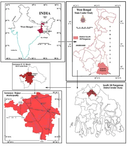
Study area
The present study selects Sonarpur-Rajpur (West Bengal, India) and its surroundings lying between 85
E. and 22024’ N. to 22026’ N. The municipality has experienced a high rate of population growth and it is one of the fastest growing cities in India. As per census from 2001, the municipality holds 3,36,628 populations with 4
and the rate of growth in this city was 3.5 per cent per annum. It has been projected in draft development report that Sonarpur-Rajpur municipality will hold nearly 0.85 million
*Corresponding author: Dr. Suman Paul,
Department of Geography, Sidho Kanho Birsha University, Purulia, West Bengal, India.
ISSN: 0975-833X
Article History:
Received 23rd March, 2017
Received in revised form 15th April, 2017 Accepted 24th May, 2017
Published online 30th June, 2017
Citation: Dr. Suman Paul, 2017. “The spatio-temporal pattern of urban growth: measurement, analysis and modelling
Research, 9, (06), 53376-53385.
Key words:
Unplanned, Shapes, Direction, RS and GIS, Monitor.
RESEARCH ARTICLE
TEMPORAL PATTERN OF URBAN GROWTH: MEASUREMENT, ANALYSIS AND
MODELLING
*Dr. Suman Paul
of Geography, Sidho Kanho Birsha University, Purulia, West Bengal, India
ABSTRACT
Urban landscape has undergone dramatic changes in most of the developing countries as a result of unplanned urban growth which needs to be analysed and understood for future planning purpose. Such growth has been facilitated by rapid development in transport and
opportunities mostly found in the surrounding regions of an urban area. This kind of growth later on takes different shapes in different directions. It can be effectively mapped and precisely analyzed with the help of statistical approach and application of RS and GIS techniques. Google map, LISS IV, Landsat images of Sonarpur-Rajpur (South 24 Parganas, West Bengal) city and its surroundings have been used to monitor the urban growth pattern during 1980 and 2010.
is an open access article distributed under the Creative Commons Attribution License, which distribution, and reproduction in any medium, provided the original work is properly cited.
process of increasing concentration of population within a town or city. It starts from a small point and after that it spreads in different directions. The growth pattern varies from one urban place to another and it is for appropriate urban planning. Urban growth can be mapped, measured and modeled by using remote sensing data and GIS techniques along with several statistical measures. The application of new techniques has created opportunities to analyse urban growth ocess which has considerable significance to understand space organization, transformation of landscape and
socio-Rajpur (West Bengal, ng between 85024’ E. to 85026’ 26’ N. The municipality has experienced a high rate of population growth and it is one of the fastest growing cities in India. As per census from 2001, the municipality holds 3,36,628 populations with 49.25 sq. km. and the rate of growth in this city was 3.5 per cent per annum. It has been projected in draft development report that
Rajpur municipality will hold nearly 0.85 million
, Sidho Kanho Birsha University, Purulia,
population in 2020. So, it will be worthwhile to monitor and quantify the urban growth pattern of Sonarpur municipality and its surroundings in order to get an idea about nature of growth, growth discrepancy and goodness or badness of growth.
Aim and Objectives
The objectives of the study are as follows
1.
To study the extent of urban growth in and around Rajpur-Sonarpur Municipality during 19802.
To find out the nature ofexpected urban growth in and around Rajpur Municipality during 1980
3.
To predict the degree of urban growth in and around Rajpur-Sonarpur Municipality for 2020 and 2030.Review of Literature
Researches on urban form till now have mostly focused on defining and quantifying urban sprawl as it has been generally accepted that urban sprawl is unplanned and cause problems for urban land use planning. Urban sprawl is so widely used a term that it has become as ambiguous as ‘compactness’ or ‘sustainable urban form’. However, the definition provided by Ewing (1997) and Paul and Dasgupta (2013) is accepted by many researchers. It states that sprawl is a condition of urban form or land uses which is char
International Journal of Current Research Vol. 9, Issue, 06, pp.53376-53385, June, 2017
temporal pattern of urban growth: measurement, analysis and modelling
TEMPORAL PATTERN OF URBAN GROWTH: MEASUREMENT, ANALYSIS AND
Purulia, West Bengal, India
landscape has undergone dramatic changes in most of the developing countries as a result of unplanned urban growth which needs to be analysed and understood for future planning purpose. Such growth has been facilitated by rapid development in transport and communication and new opportunities mostly found in the surrounding regions of an urban area. This kind of growth later on takes different shapes in different directions. It can be effectively mapped and precisely analyzed with roach and application of RS and GIS techniques. Google map, LISS IV, Rajpur (South 24 Parganas, West Bengal) city and its surroundings have been used to monitor the urban growth pattern during 1980 and 2010.
ribution License, which permits unrestricted use,
population in 2020. So, it will be worthwhile to monitor and quantify the urban growth pattern of Sonarpur-Rajpur municipality and its surroundings in order to get an idea about th, growth discrepancy and goodness or badness
The objectives of the study are as follows
To study the extent of urban growth in and around Sonarpur Municipality during 1980 – 2010, To find out the nature of discrepancy in actual and expected urban growth in and around Rajpur-Sonarpur Municipality during 1980 – 2010 and
To predict the degree of urban growth in and around Sonarpur Municipality for 2020 and 2030.
Researches on urban form till now have mostly focused on defining and quantifying urban sprawl as it has been generally accepted that urban sprawl is unplanned and cause problems for urban land use planning. Urban sprawl is so widely used a s become as ambiguous as ‘compactness’ or ‘sustainable urban form’. However, the definition provided by Ewing (1997) and Paul and Dasgupta (2013) is accepted by many researchers. It states that sprawl is a condition of urban form or land uses which is characterized by low-density,
INTERNATIONAL JOURNAL OF CURRENT RESEARCH
Fig.1. The Location of the Study Area
Table 1. Data used for the study
Type of Data used Year I.D. (Topo. No./ path/row) Scale/ Resolution No. of bands Source
Toposheet 1978 73F/7 1:50000 ---- Survey of India
Landsat TM 1980 151/ 41 28.5 m. 4 Landsat.org
Landsat TM 1990 101/ 85 28.5 m. 7 Landsat.org
Landsat ETM+ 2000 101/ 85 28.5 m. 7 NRSA
Google Map 2010 --- 1:1 True Colour Composite Google Pro. (Open Source)
Sonarpur-Rajpur Municipality Map
2005 -- 1” to 10’ -- Municipality Office
Table 2. Built-up Area (sq. km.) of Sonarpur-Rajpur and Its Surroundings during 1980 – 2010
Year Directions Total Area
in Sq. Km.
NW NE SE SW
1980 16.85 4.3 1.8 5.2 28.15
1990 20.61 6.45 2.39 8.41 37.86
2000 28.43 9.27 7.25 12.35 57.3
2010 35.72 18.46 9.61 15.17 78.96
[image:2.595.173.420.713.775.2]scattered development; commercial strip development, and leapfrog (i.e. discontinuous) development. Sprawl, by definition, is a condition (some researchers prefer ‘process’) of urban form, and in this paper the measures and indices have been developed to quantify urban sprawl as a representative of urban form. It should be kept in mind that limited attempts have been made to analyze and quantify the urban form; most of the studies have been carried out so far to quantify the sprawling and compactness of urban form. Before the discussion on the quantitative measures of urban form, it is necessary to clarify its meaning. Generally, urban form refers to the physical structure of an urban area. It has also been indicated as the spatial pattern of human activities at a certain point of time (Anderson et. al. 1996). Urban form can be viewed from aggregate and disaggregate standpoints. The former indicates to the overall three dimensional structure of the urban area (settlement size and density) and the latter looks into the spatial pattern within the urban area. Urban form can be viewed from different geographical scales- regional (Fina and Siedentop, 2008), country (Cirilli and Veneri, 2008), metropolitan (Bertaud and Malpezzi, 1999; Paul and Dasgupta, 2013).
Significant number of studies has been conducted to find out the measures and indices to quantify sprawl. Still, contentions are in place as to which technique can best explain the urban compactness or sprawl. Such approaches can be broadly grouped in two types- those who identify the sprawl as a ‘process’ and those recognize sprawl as a ‘condition’ of urban form. The present study is about quantifying and analyzing a particular urban area, so it considered the second set of studies. The most widely used measure of urban form is density, measured by the land consumption per capita. Torrens and Alberti (2000) determines the density level at which the urban form can be considered as sprawling. But density or settlement size can only provide the aggregate measure of urban form. Galster et al. (2000) suggested seven other measures, in addition to density, to quantify the compactness of urban form at the disaggregate level. These include- continuity, concentration, clustering, centrality, nuclearity, mixed uses and proximity. Many researchers have also employed one or more of these indicators to explain the urban form. Tsai (2005) suggests Gini coefficient and Moran coefficient (also called Moran’s I) to measure the distribution and clustering of urban place respectively. Interestingly, Moran’s I can also measure ‘continuity’ and ‘nuclearity’ Galster et al. (2000). So this study selected the Gini and Moran co-efficients to quantify the urban form. Centrality and Proximity are closely linked. Fractal dimension (Terzi and Kaya, 2008) and total core area index (Fina and Siedentop, 2008) refer to the geometric aspects of urban form, not the activity or land use distribution, so they were also excluded from this analysis.
MATERIALS AND METHODS
Data used
In order to study the spatial pattern and extent of sprawl during 1980 – 2010 in the study area, SOI sheets (73 F/7) with the scale of 1:50000 of 1978 have been considered for georegistration purpose. Landsat TM (P/R: 151:43) for 1980, Landsat TM (P/R: 140/44) for 1990 and Landsat ETM+ (P/R: 140/44) for 2000 satellite images have been taken into account. To identify the current scenario of the study area, Google Image of the study has been considered.
Methods
Classification of Images
eCognition Developer 8 software has been used for image classification due to the advantage of classifying image on object level instead of pixel level. Object-oriented classification avoids mixed pixel problems which usually occur in urban area image classification. The images were obtained as standard product that is, geometrically and radiometrically corrected. However, due to the different standards and references used by the image supplying agencies, the overlay of the images does not match with
considerable accuracy. To solve this problem, images were co-registered so that the overlay matches with sub-pixel
accuracy (root mean square errors=0.21). Nearest-neighbour resampling method was used to transform the images so that the original pixel value retains. Ten years variations of built-up areas were extracted from the classified images, from which we can assess the dynamic changes of urban growth in Sonarpur-Rajpur and its surroundings. For the Landsat TM images, the built-up areas were extracted after image processing and image classification and then built-up areas were regarded as one of the indicators to measure urban growth.
Built-up Index
Built-up Index is also a good indicator for monitoring the changes of land use and land cover. The built-up index is
computed for the year of 1980, 1990, 2000 and 2010 from near-infrared (0.78-0.90 μm) and middle-infrared (1.55-1.75
μm) by using the following formula (Dolui G et. al., 2014) :
BUI = (MIR – NIR) / (MIR + NIR)
Chi-square Analysis
Observed urban growth has to be compared with expected urban growth to understand nature of discrepancy in urban growth. In this study Chi-Square analysis has been performed to find out the degree of freedom (Chi-Square value). The chi-square has a lower limit of 0, when the observed value exactly equals the expected value. Higher the chi-square (degree-of-freedom) value, more the discrepancy between actual and expected urban growth.
Shannon’s Entropy
Shannon’s entropy is a well-accepted method for determining the sprawled urban pattern (Kumar et al., 2007; Lata et al., 2001; Li & Yeh, 2004; Sudhira et al., 2004; Yeh & Li, 2001). This value ranges from 0 to log n, indicating very compact distribution for values closer to 0. The value closer to logn indicates that the distribution is much dispersed. Larger value of entropy reveals the occurrence of urban sprawl.
Degree of Goodness
Since the chi-square of-freedom) and entropy (degree-of-sprawl) are different measures and one may contradict other
in some of the instances (as it is evident in this study), it necessitates determining the ‘degree-of-goodness’ of the
growth relates the expected growth and the magnitude of compactness (as opposed to sprawl).
Modelling Urban Growth
The urban growth model has been designed and developed to predict the growth pattern of Sonarpur-Rajpur municipality.
Fig.2. The Methodology in Flowchart
In order to explore the probable relationship of percentage built-up (dependent variable) with causal factors of urban built-up (α-population, β-population densities, etc.), regression analysis was undertaken. Various regression analyses (linear, quadratic, exponential and logarithmic) were carried out to ascertain the nature of significance of the causal factors (independent variables) on the sprawl, quantified in terms of percentage built-up.
RESULTS
Extent of Urban Growth
The classification of satellite images into built-up (along with other impervious) and non-built-up areas during 1980-2010 have produced abstracted and highly simplified visual images in the study area (Figure 3a-3d.) which define the urban extents of specified times. Examining four classified images, even curiously, one can see that expansion of the city in the specified zones of the study area has different signatures: some zones are very compact while others have more open spaces between built-up areas. In some areas the boundary between built-up and non- built-up portion is sharp, while in other areas urban and non-urban part cannot be segregated. By interpreting these imageries, one can easily understand whether the area is becoming more monocentric or polycentric over time. Surely, one can grasp these patterns intuitively, but they fall short of providing solid evidences for debating and deciding upon the future growth of the city. To describe these different patterns intelligently and to understand how they change over time or to compare each zone with others and to explain the variations among these patterns there is a need to select appropriate quantitative measures which can satisfactorily answer the above mentioned queries
Built-up Area and Urban Growth
The percentage of an area covered by impervious surfaces such as asphalt and concrete is a straight forward measure of urban growth (Barnes et al., 2001). It can safely be considered that developed areas have greater proportions of impervious surfaces compared to the lesser-developed areas (Sudhira et al., 2004; Paul and Dasgupta, 2013).
Table 3. Observed Growth of Sonarpur-Rajpur and Its Surroundings during 1980 – 2010
Temporal Span Directions Column
Total
NW NE SE SW
1980 – 1990 3.76 2.15 0.59 3.21 9.71
1990 – 2000 7.82 2.82 4.86 3.94 19.44
2000 – 2010 7.29 9.19 2.36 2.82 21.66
Row Total 18.87 14.16 7.81 9.97 50.81
Source: Computed by Authors from Table 2.
The built-up areas for each zone and for each temporal instant are furnished in Table 2 that directly shows the status of built-up areas in the Rajpur-Sonarpur municipality and its surroundings. Table 2 indicates the built-up area of the municipality and changes over the time in different directions. Observed growth in built-up area (Table 3) has been calculated for the time spans 1980–1990, 1990–2000 and 2000–2010. The percentage of increase in built-up area has also been calculated (Table 4)
Table 4. Observed Growth Rate of Sonarpur-Rajpur and Its Surroundings during 1980 – 2010
Temporal Span
Directions Column
Total
NW NE SE SW
1980 – 1990 22.31 50.00 32.78 61.73 34.49
1990 – 2000 37.94 43.72 203.35 46.85 51.35
2000 – 2010 25.64 99.14 32.55 22.83 37.80
Source: Computed by Authors from Table 3.
This clearly shows that the rate of urban growth is fluctuating with time and all the zones have achieved maximum observed growth rate during 2000-2010. But this finding does not necessarily indicate that there is a ‘compact’ or ‘good’ development of built-up area in the city and its surroundings and therefore it needs further analysis.
Analysis of differences between observed and expected urban growth through chi-square analysis
Observed growth ought to be compared with expected growth for the understanding of discrepancy. Table 3 shows the observed growth in urban land-cover. From this table, the theoretical expected urban growth can be calculated statistically by employing the Eq. (1). Let the Table 3 be called matrix UG, with elements UGij, where i = 1, 2... n (specific time span of analysis, rows of the table) and j= 1, 2, .., m (specific zone, columns of the table). The expected built-up growth for each variable was calculated by the products of marginal totals, divided by the grand total (Almeida et al., 2005). Therefore, the expected growth UGij for the ith row and jth column is:
= --- ……….. (1)
where, = row total, = column total and = grand total = ∑ ∑ = UGij
Table 5. Expected Urban Growth Rate in Different Direction during 1980 – 2010
Temporal Span Directions
NW NE SE SW
1980 – 1990 3.61 2.71 1.49 1.91
1990 – 2000 7.22 5.42 2.99 3.81
2000 – 2010 8.04 6.04 3.33 4.25
[image:6.595.306.559.87.149.2]Source: Computed by Authors.
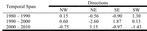
Table 6. Differences between actual and Expected Urban Growth Rate during 1980 – 2010
Temporal Span Directions
NW NE SE SW
1980 – 1990 0.15 -0.56 -0.90 1.30
1990 – 2000 0.60 -2.60 1.87 0.13
2000 – 2010 -0.75 3.15 -0.97 -1.43
Source: Computed by Authors.
Pearson’s chi-square statistics takes into account the checking of freedom amongst pairs of variables chosen to explain the same category of land-cover change (Almeida et al., 2005; Paul and Dasgupta, 2013). Therefore, to determine the ‘degree-of-freedom’, chi-square (χ2) test was performed with the Pearson’s chi-square expression: (observed – expected)2/ expected. It reveals the freedom or degree of deviation for the observed urban growth over the expected. For Table 3 (observed) and Table 5 (expected), the chi-square (χ2) statistics for each temporal span was calculated as (Table 7):
( − )2
χ = ∑ --- ……….. (2)
where,
χ =
degree of freedom for the ith span, = observed built-up area in jth column for a specific row and = expected built-up area in jth column for a specific row. Now, if we replace j (column) by i (row), and m (number of columns) by n (number of rows) in Eq. 2, we can determine the degree-of-freedom for each zone also.The chi-square has a lower limit of 0, when the observed value exactly equals the expected value. Table 7 clearly shows that the degree-of-freedom is low (i.e., similarity in observed and expected values) for both of the temporal spans. Table 7 shows that the freedom is low (i.e., similarity in observed and expected values or very near) for only NW whereas it is high for SE, SW and NE. Needless to say, the overall degree-of-freedom is extremely low to moderate. Lower overall degree-of-freedom indicates equal weightage and consistency in planning with the entire city in consideration. Lower degree-of-freedom for a zone is an indication of stable development within the zone with the change of time. Again lower degree-of-freedom for a temporal span can be considered as lower inter-zone variability in urban growth. However, it is worth mentioning that lower degree-of-freedom can be considered as sprawl, instead it should not be considered as disparity in growth as a process and/or pattern. This method of analysis is a new approach and essentially adds knowledge to the similar existing literature. Bonham-Carter (1994) and Almeida et al. (2005) have used chi-square for determining the overall freedom; but the present paper shows how this model can be used to analyse the urban growth in three different dimensions (pattern, process, and overall).
Table 7. Degree-of-Freedom for Urban Growth for Each Zone and Each Temporal Span
Temporal Span Directions Column
Total
NW NE SE SW
1980 – 1990 0.01 0.11 0.55 0.89 1.56
1990 – 2000 0.05 1.25 1.17 0.00 2.47
2000 – 2010 0.07 1.65 0.28 0.48 2.48
Row Total 0.13 3.01 2.00 1.38
Source: Computed by Authors.
Shannon’s Entropy and Urban Growth
Shannon’s entropy is a well-accepted method for determining the sprawled urban pattern (Yeh & Li, 2001; Lata et al., 2001; Li & Yeh, 2004; Sudhira et al., 2004; Kumar et al., 2007; Paul & Dasgupta, 2013). In this study, the Shannon’s entropy for each temporal span (Hi) has been calculated from Table 4 by using the following formula:
Hi=
∑
Pj loge (Pj) ……….. (3)where, Pj = proportion of the variable in the jth column (i.e., proportion of built-up growth rate in jth zone, calculated (from Table 4) by: built-up growth in jth zone/ sum of built-up growth rates for all zones) and m= number of zones= 4).
[image:6.595.38.282.192.244.2]The degree-of-sprawl can be identified by magnitude of entropy value. The value of entropy ranges from 0 to loge(m). Value 0 indicates that the distribution of built-up is compact, while values closer to loge(m) reveal that the distribution of built-up is dispersed. Higher values of entropy indicate the occurrence of sprawl.
Table 8. Shannon’s Entropy Analysis (Zone Wise)
Zones NW NE SE SW
Entropy (Hi) 0.37 0.36 0.29 0.32
loge (m) --- 1.39 ---
loge (m)/2 --- 0.69 ---
Source: Computed by Authors.
[image:6.595.307.558.461.503.2]demonstrates how the entropy model can be used in three different temporal dimensions for the analysis of urban growth. This new approach is expected to be appreciated in addition to the existing literature (Bhatta, 2009a; Kumar et al., 2007; Lata
et al., 2001; Li & Yeh, 2004; Sudhira et al., 2004; Yeh & Li,
2001) that uses the entropy to evaluate the sprawl as a pattern only.
Degree of goodness
Since the chi-square of-freedom) and entropy (degree-of-sprawl) are different measures and one may contradict other in some of the instances (as it is evident in this study), it necessitates determining the ‘degree-of-goodness’ of the urban growth. The degree-of-goodness actually refers to the degree at which observed growth relates to the expected growth and the magnitude of compactness (as opposed to sprawl). This can be calculated for each temporal span as (Table):
1
Gi = loge [ ---] ……….. (4)
χ2 ( Hi )
loge(m)
where, Gi =degree-of-goodness for i-th temporal span, χ2= degree-of-freedom for ith temporal span, Hi =entropy for ith temporal span, m= total number of zones = 4. The degree-of-goodness for each zone (Table 9) can also be calculated if we replace i by j and m by n in the Eq. (4). Overall degree-of-goodness can be calculated as:
1
Gi = loge [ ---] ……….. (5)
χ2 ( H i )
loge(n)
Where, χ2 is overall freedom and H is overall sprawl.
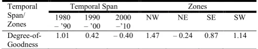
[image:7.595.31.293.640.683.2]Degree-of-goodness is a straightforward measure; positive values indicate ‘goodness’ whereas negative values indicate ‘badness’. The degree-of-goodness (or badness) can also be identified by the magnitudes from Table 10. This analysis shows how the goodness varies in different zones and in different temporal spans, or whether the goodness is positive or negative. From this analysis it can be said that, during the time span 1980–‘90, the city has experienced high ‘goodness’ in urban growth. Analysis of individual zone also reveals similar conclusion; although NW, SW and SE have shown positive value, however but a negative value can be seen in NE only. The overall degree-of-goodness is quite impressing.
Table 9. Shannon’s Entropy Analysis (Temporal Span Wise)
Temporal Span 1980 – 1990 1990 – 2000 2000 – 2010
Entropy (Hi) 0.32 0.37 0.36
loge (m) --- 1.39 ---
loge (m)/2 --- 0.69 ---
Source: Computed by Authors.
Table 10. Degree-of-Goodness (Direction/ Zone and Temporal Span wise)
Temporal Span/ Zones
Temporal Span Zones
1980 – ’90
1990 – ’00
2000 –’10
NW NE SE SW
Degree-of-Goodness
1.01 0.42 – 0.40 1.47 – 0.24 0.87 1.14
Source: Computed by Authors.
Modelling Urban Growth
Linear, quadratic (order = 2), and logarithmic (power law) regression analyses were tried and the results are tabulated in Annexure. All these regression analyses reveal the individual contribution by the causal factors on the urban growth. The most significant relationships are outlined in Eqs. (6)–(10). The linear regression analyses revealed that the population has a significant influence, which is evident from the x coefficient. The quadratic regression analyses for second order revealed that the β-population density and distance from urban centre (Kolkata) have a considerable role in the urban growth phenomenon. It is evident from the result that the urban growth declines with increase in distance from Kolkata. The logarithmic (power law) regression analyses revealed that the β- population density has influenced the urban growth phenomenon, which is evident from the value of exponent. Positive value of the exponent infers that built-up area increases exponentially with increase in popaden (α-population density). The probable relationships are,
Pcbuilt2020 = 0.000811 × pop2011 +9.87149 (r = 0.6749) ... (6)
Pcbuilt2020 = 0.007641 × (popbden) 2
− 1.2 × 10⁻⁷×(popbden) + 5.8950 (r = 0.8823) …….… (7)
Pcbuilt2020 =−1.6953 × (Koldist)2 + 0.02593×(Koldist) + 35.8807 (r = 0.60) …………. (8)
Pcbuilt2020 =−0.8017 × (Baruidist)2 + 0.002242×(Baruidist) + 12.9731 (r = 0.683) ...…. (9)
Pcbuilt2020 = 0.370 × (popaden)1.6938 (r = 0.4779)…….. (10)
where, Pcbuilt = built-up in 2020, pop2011 = 2011 Population, popaden = α-population density, popbden = β-population density, Koldist = Distance from Kolkata, Baruidist = Distance from Baruipur and AGR =Annual growth rate of Population. To assess the cumulative effects of causal factors, stepwise regression analysis considering multivariate was done. In the multivariate regression it is assumed that the relationship between variables is linear.
Pcbuilt =−21.7633+ pop2011×− 0.12529 + agr ×− 0.0004 + popaden × 0.00642 + popbden×0.5289 + Koldist × 0.7451 + Baruiidist× -0.00139 (r = 0.86) ……… (11)
Considering all the causal factors in the stepwise regression, Eq. (11) indicates the highest correlation coefficient. The anomaly in considering Eq. 6-10 for prediction is that, popaden is nothing but the population density of Sonarpur-Rajpur municipality to the built-up area of that area. However, the relationships 7–10 confirm that the causal factors collectively have a significant role in the built-up phenomenon, as can be understood from the positive correlation coefficients.
DISCUSSION
[image:7.595.29.295.737.788.2]directs us to divide the study area in four square sections. However, one may divide it in more (or even less) subsections than the demonstrated one. Furthermore, the study area can also be divided into circular zones, or preferably both in circular and square. This will certainly provide a better insight into the urban growth of the city and its surroundings. Different zones have a different level of compactness leading to different patterns of growth; therefore, a single policy for the entire city never works with equal degree of effectiveness for all. However, since the main aim of this study was to introduce new methods of analysis, rather than the exhaustive study on the city, only four square sections were considered. It may be mentioned that if one divides the city into circular zones in addition to pie sections, the distance to the central business district from a specific zone will indirectly be accounted, which may be desired by many proponents. The distance to the central business district is an important consideration since the urban density changes with it. This study considers a square area equidistant from the city-centre. It assumes that the possibility of growth is equal in every direction from the city-centre; since it does not consider road network, distribution of commercial centres or other variables that may cause uneven growth. However, it is not essential to consider a square area; instead, the natural boundary or urban extent can also be considered and be divided into several parts. Administrative boundaries (although they do not properly reflect the dynamics of urban expansion) can also be considered which can reflect socio-economic dependencies/ independencies. Natural boundaries rarely have the data on socioeconomic variables. In most of the countries, including India, data on these variables are available in respect of
administrative boundaries. Bhatta (2009) considers the administrative boundary of Kolkata, subdivided into five
parts, to analyse the urban growth pattern in consideration of socio-economic variables and Shannon’s entropy. The demonstrated models of current research are not directly dependent on how the study area has been considered or how it has been divided. They also do not depend on the number of divisions. Obviously, more number of divisions gives the opportunity for more detailed analysis resulting in more reliability.
The measures employed in this paper are based on built-up areas in each zone. However, land areas available for development in each zone are not same. Therefore, it would be better if the three measures (freedom, sprawl, and goodness) could be calculated on the basis of percentage of built-up area within a zone by excluding non-developable land. This percentage can be calculated by the following formula: [{built-up area within a zone/ (total area of the zone - non-developable land within the zone)} x 100]. However, area of non-developable land cannot be measured directly from the remote sensing data. An area may be non-developable for several reasons that include natural (river, rugged terrain), ownership (land owned by military), government policy (to preserve an open space, water body, or agriculture), legal disputes on land, and several others. Therefore, it may be difficult to get such temporal dataset. However, if these data are available, one may proceed by considering the aforementioned percentage of built-up data; and obviously will get more reliable results. The approach of this study may be criticized due to its simplified approach for the analysis of urban growth pattern. Several arguments can be made due to non-consideration of road network, distribution of commercial centres, terrain properties, transition among different land-uses, and many more that have
been explained by the researchers as mentioned in the introduction. But, one has to remember that, in developing countries, cities have grown with unplanned developmental initiatives. In many instances, these cities lack historical data of urban development and temporal inventory of land-use/land-cover data. Therefore, many of the spatio-statistical models cannot be adopted for these cities. Furthermore, in several instances (as for the Sonarpur-Rajpur Municipality), the city administrators are not well conversant with the new tools or methods and modern technologies such as geospatial technology. Therefore, they demand simple analytical approaches that require minimal set of input data. The demand of simplicity arises from this point of view, and needless to say, the proposed approach would be very helpful in terms of its easy methods of deriving historical data from satellite imageries and also in terms of statistical analysis.
In this study, the demonstrated approach of determining the goodness, however, had a major limitation did not take into account any policy variables of the past. It is worth mentioning that although in the industrialized countries they may have proper planning policies for their cities; however, the cities in developing countries lack such type of policies in most of the cases and they grow with all freedoms. Therefore, the demonstrated approach will be very useful for the cities in developing countries. However, this does not mean that the proposed model to quantify the degree-of-goodness cannot be used for the cities in industrialized countries. In this study the expected urban growth was calculated by a statistical approach (Eq. (1)) based on the past and present urban growth, since there was no such predetermined and planned expectations. In many of the cities of industrialized countries, they have predetermined and preplanned expectations of urban growth. Therefore, for this city and its surroundings, instead of considering the Eq. (1), we should consider the predetermined values. And thus, the quantification of degree-of-freedom and degree-of-goodness will be influenced by the policy variables.
Conclusion
The study was aimed to analyse the urban growth from remote sensing data with a new approach. Several statistical and mathematical models have been applied for studying the urban growth as a process, pattern, and the overall condition as well. The analysis has resulted in several matrices for understanding the urban growth in the Sonarpur-Rajpur municipality and its surroundings. The analysis shows that the city has a general moderate to low degree-of-freedom and it is non-sprawling in nature, however, the tendency compactness is increasing with time although the of- freedom is lowering. The degree-of-goodness is not alarming. It can also be concluded that the goodness of urban growth, for the study area, is increasing due to inclining urban growth rate. This study would be helpful for the local authorities and proponents in terms of guiding future planning and policy-making, and for debating. The models demonstrated in the preceding sections, driven by remote sensing data and GIS, have proved to be useful for the identification of urban growth pattern and their general tendencies. A new model, degree-of-goodness and prediction analysis has also been introduced in this study which can analyse the urban growth in a single measurement scale. Two other statistical models-Pearson’s chi-square statistics and Shannon’s entropy have also been used in a new approach that can result in a more detailed data for the analysis of urban growth. The demonstrated models are empirically devised approaches and not constrained by the strait jacket of rigid theory devices; therefore, they can be applied on other cities as well, especially in developing countries. A new hypothesis can be derived from the preceding analysis and discussion-‘‘degree-of-goodness is an indicator of sustainable development’’, which may serve the purpose of future analysis and research.
In summary, this study opened with an observation about the important roles of analytic models for urban growth by using remote sensing data, proceeded to use some statistical and mathematical models and to propose a new model. It also focuses the scope of research and application for the city planners and proponents in developing nations as well as worldwide. The theory and models of urban growth analysis which are supported by preceding findings should prove useful in devising policy responses for the future research and application on urban growth by using the demonstrated models for the city planners and administrators.
REFERENCES
Anderson, W. P., Kanaroglou, P. S. and Miller, E. J. 1996. Urban form, energy and the environment: a review of issues, evidence and policy, Urban Studies, 33 (1), pp. 256 - 271.
Bertaud, A. and Malpezzı, S. 1999. The Spatial Distribution of Population in 35 World Cities: The Role of Markets, Planning and Topography, Center of Urban Land Economics Research, The University of Wisconsin, WI, USA.
Bhatta, B. 2009b. Spatio-temporal analysis to detect urban sprawl using geoinformatics: A study of Kolkata”. Proceedings of 7th All India Peoples’ Technology Congress, Kolkata, 06–07 February, Forum of Scientists, Engineers & Technologists.
Bhatta, B., S. Saraswati and D. Bandyopadhya, 2010. “Quantifying the degree-of-freedom, degree-of sprawl and
degree-of-goodness of urban growth from remote sensing data”. Journal of Applied Geography, 30 (2), pp. 96–111. Brueckner, Jan K. and David A. Fansler, 1983. “The
Economics of Urban Sprawl: Theory and Evidence on the Spatial Sizes of Cities”. The Review of Economics and
Statistics, 65 (3), pp.136–144.
Cirilli, A. and Veneri, P. 2008. “Spatial structure and mobility patterns: Towards taxonomy of the Italian urban systems”. Economic Papers. http://dea.univpm.it/quaderni/pdf/313. pdf (accessed on July 14, 2015).
Civco, D. L., Hurd, J. D., Wilson, E. H., Arnold, C. L., and Prisloe, M. 2002. “Quantifying and describing Urbanising Landscapes in the Northeast United States”. Photogrammetric Engineering and Remote Sensing, 68 (10), pp. 1083-1090.
Dasgupta A and Paul S 2013. “Analysis of Urban Growth using RS, GIS and Shannon's Entropy in and around Burdwan City, West Bengal, India”. Indian Journal of
Spatial Science, Vol - 4.0 No. 2 Winter Issue 2013. pp. 71
– 80.
Dolui G et al. 2014. “An application of Remote Sensing and GIS to Analyze Urban Expansion and Land use Land cover change of Midnapore Municipality, WB, India”.
International Research Journal of Earth Sciences, Vol.
2(5), pp. 8-20
Ewing, R. 1997. “Is Los Angeles-style sprawl desirable? Journal of the American Planning Association”, http://stuff.mit.edu/afs/athena/course/11/11.951/albacete/C ourse%20Reader/Transportation/High-Speed%20Tranist% 20Literature%20Review/Ewing%201997.pdf. (Accessed on July 6, 2015).
Fang S., Gertner G. Z., Sun Z. and Anderson A.A. 2005. “The Impacts of Interactions in Spatial Simulation of the Dynamics of Urban Sprawl”. Landscape and Economic Planning, 73 (4), pp. 294-306.
Fina, S. and Siedentop, S, 2011. “Urban sprawl in Europe – identifying the challenge”. REALCORP, Vienna. http://programm.corp.at/cdrom2008/papers2008/CORP200 8_34.pdf.(Accessed on May 11, 2012).
Galster, G. et al. 2000. “Wrestling Sprawl to the Ground: Defining and Measuring an Elusive Concept. Housing Policy Debate, Vol. 12, pp. 681-717. www.mi.vt.edu/data/ files/hpd%2012(4) /hpd% 2012(4) galster.pdf (accessed on July 21, 2012).
Herold, M., Goldstein C.N. and Clarke, C.K. 2003. "The spatiotemporal form of urban growth: measurement, analysis and modeling". Remote Sensing Environment, 86 (2), pp. 286-302.
Husain, I. and Siddiqi L. 1979. “Urban Encroachment on Rural Lands: A Case Study of Modinagar”. The Geographer, Aligarh, 6 (1), pp. 11-21.
Jensen, J. R. & Cowen, D. C. 1999. “Remote sensing of urban/suburban infrastructure and socioeconomic attributes”. Photogrammetric Engineering & Remote Sensing, Vol. 65, pp. 611–622.
John E. Hasse and Richard G. Lathrop, 2003. “Land resource impact indicators of urban sprawl” Applied Geography, 23 (1), pp. 159–175.
Jothimani, P. 1997. “Operational urban sprawl monitoring using satellite remote sensing: excerpts from the studies of Ahmedabad, Vadodara and Surat, India”. Paper presented at 18th Asian Conference on Remote Sensing held during October 20–24, Malaysia.
case study of Indore city”. Journal of Indian Society of
Remote Sensing, 35(1), pp. 11–20.
Kundu, A et al. 2002. “Dichotomy or continuum-Analysis of impact of urban centers on their periphery”. Economic and Political Weekly, XXXVII (50), pp. 1786 - 1797.
Lata, K.M. et al. 2001. “Measuring urban sprawl: a case study of Hyderabad”, GIS Development 5, (12), pp. 439 - 456. Liu J. and X. Deng, 2004. "An Overview of Urban Land
Expansion in China in the 1990s Based on Remote Sensing and GIS Technologies," Geographical Review of Japan,
77, pp. 800-812.
Md. Shakil Bin Kashem et al. 2009. “Quantifying Urban form: A Case Study of Rajshahi City”, Journal of Bangladesh
Institute of Planners, 2, pp. 39-48.
Michael Oloyede ALABI, 2009. “Urban sprawl, pattern and measurement in Lokoja, Nigeria” Theoretical and
Empirical Research in Urban Management, 4 (19), pp.
158-164.
Paul S and Dasgupta A. 2013. “Spatio-temporal analysis to quantify urban sprawl using Geoinformatics”. Int. Journal
of Advances in Remote Sensing and GIS, Vol. 1, No. 2, pp.
234 – 248.
Prakasam. C. 2010. “Land use and land cover change detection through remote sensing approach: A case study of Kodaikanal taluk, Tamilnadu. International Journal of
Geomatics and Geosciences, Vol. 1 (2), pp. 150-158.
Ronghua Ma et al. 2008. “Mining the Urban Sprawl Pattern: A Case Study on China”, Applied Geography, Vol. 21 (2), pp. 6371-6395.
Saikia, B. and Bezbarua, M.P. 1995. “Impact of urban centre on Rural Economy- a case study of three villages in Hajo-circle near Guwahati city”, Assam Economic Review,
IV,V,VI, Dept. of Economics, G.U. Assam.
Saravanan. P and Ilangovan, P. 2010. “Identification of Urban Sprawl Pattern for Madurai Region Using GIS”.
International Journal of Geomatics and Geosciences, 1 (2),
pp. 141-149.
Sudhira H. S. et al. 2004. “Urban sprawl: metrics, dynamics and modelling using GIS” International Journal of Applied
Earth Observation and Geoinformation, 5. pp. 29–39
Sudhira, H.S., T.V. Ramachandra and K.S.Jagadish, 2004. “Urban sprawl: metrics, dynamics and modelling using GIS”. International Journal of Applied Earth Observation
and Geoinformation, 5 (1), pp. 29–39.
Tamilenthi S. et al. 2011. “Dynamics of urban sprawl, changing direction and mapping: A case study of Salem city, Tamilnadu, India”. International Journal of
Geomatics and Geosciences, 3 (1), pp. 277-286.
Terzi, F. and Kaya, H. S. 2008. “Analyzing Urban Sprawl Patterns through Fractal Geometry: The Case of Istanbul Metropolitan Area”. Working Paper Series, Paper-144, CASA: Centre for Advanced Spatial Analysis, University College London, London.
Torrens P. M. and Alberti, M. 2000. “Measuring Sprawl”. Working Paper Series, Paper-27, CASA: Centre for Advanced Spatial Analysis, University College London, London.
Tsai Y. H. 2005. “Quantifying urban form: compactness versus ‘sprawl”. Urban Studies, Vol. 42(1), pp. 141-161. http://www.webs1.uidaho.edu/ce501-400/resources/tsai. p.d.f. (accessed on August 8, 2015).