On the Alternative Approach to Active Control

(1)

ISSN Online: 2327-4379 ISSN Print: 2327-4352

DOI: 10.4236/jamp.2018.611191 Nov. 22, 2018 2303 Journal of Applied Mathematics and Physics

On the Alternative Approach to Active Control

Vladimir V. Arabadzhi

Division of Geophysical Research, Institute of Applied Physics (RAS), Nizhny Novgorod, Russia

Abstract

Paper is devoted to problem of acoustical visibility reduction and gives brief description of alternative approach to active control. This approach allows sa-tisfy jointly the four conditions: a) effective suppression of acoustical radia-tion and scattering caused by elastic body immersed in compressible medium (water); b) cloacking at any important temporal frequencies of observant sound waves; c) cloacking at any important spatial frequencies or at any ob-servation directions; (d) thickness of the masking shell is much smaller than the length of suppressed waves. Technological development gives more and more fast and miniature control elements and fast, accurate calculations. On the other hand, the lengths of waves to be damped are constant due to the constant conditions of their far propagation. The approach suggested uses operations of high space-time resolution for long waves controlling. Because the joint fulfillment of the conditions of acoustic support absence and the thinness of the shell and also the causality of control lead to the need to oper-ate at frequencies of much higher than frequencies of waves to be damped. It is assumed that the incident waves are represented by a discrete set of plane waves of finite duration. Also it is assumed only that the characteristic spatial scale of the distribution of normal velocities on the surface of the protected body is limited from below. The boundary value problem with initial condi-tions is considered.

Keywords

Boundary and Initial Conditions, Flat Impact, Flat Imprint, Imprint Relaxation, Depth of Imprint, Transparent Supportless Unidirectional Sources of Acoustical Wavelets, Leading Edge of Incident Wave, Leading Pair of Microphones

1. Introduction

Modern results [1] in the field of cloacking correlate with the famous article [2]. In this paper, an analytical solution is obtained in the case when the incident

How to cite this paper: Arabadzhi, V.V. (2018) On the Alternative Approach to Active Control. Journal of Applied Mathe-matics and Physics, 6, 2303-2312.

https://doi.org/10.4236/jamp.2018.611191

(2)

V. V. Arabadzhi

DOI: 10.4236/jamp.2018.611191 2304 Journal of Applied Mathematics and Physics wave is flat and monochromatic, and the body has a spherical shape. The solu-tion of this problem is tangentially homogeneous radial distribusolu-tion of medium parameters in the outer spherical layer (that is the time-constant distribution of the passive parameters of the medium in the masking shell). Thus, the distribu-tion of parameters required for the masking inside the protective layer depends on the frequency of the incident wave and does not depend on the direction of arrival of the incident wave. The need to adjust the spatial structure of the masking shell to a nonplanar form and the given direction of the incident wave (or to the non–spherical shape of the body) even in the monochromatic case, makes the practical application of the solution extremely complicated. Moreover the dynamic range of mechanical vibrations of the elements of the masking shell can be significantly exceeded, since all the power of the incident wave through the cross section of the protected body must tangentially pass inside the shell, the thickness of which we seek to reduce (see abstract, (d)). In addition, the above-described shell is not designed to suppress the radiation of the protected body. We will consider below the possibilities of radiation and scattering sup-pressing for all directions of observation and for all directions of the incident waves in the ranges ωmin≤ ≤ω ωmax_and

max min max min

2 /π ωc =λ ≤ ≤λ λ =2 /π ωc _{of frequencies and wavelengths (where}

min

ω _,ω_max_, λ_min_, λ_max_{sound damping range boundaries,}_c_{–sound speed in}

outside compressible medium) under the broadband ωmin<<ωmax , min

/λ 1

Ξ >> _{, and}Ξ/λ_max <<1_{, where}Ξ_{–characteristic linear dimension of} body protected with convex smooth surface SB) and small thickness 2 h_{of the}

active shell (coating between inner and outer surfaces SB and S) of the

pro-tected body in comparison with the lengths of quenched waves, i.e. 2h<<λmin.

And the forced condition of inflexibility of surface SB for spatial scales min >>λmin/ 2

 on any frequency ω.

2. Radiation Suppression

In the most general formulation, we need to create on the active shell surface S a predetermined distribution U•( , )rt (r∈S) of the normal displacements of particles, despite the action of unknown sources of vibrations inside the surface

B

S .In particular, to suppress radiation, we need to create U•( , ) 0rt = , i.e. no incident waves.

2.1. Shock Molding of Desired Boundary Form

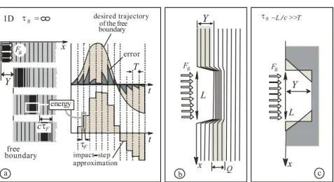
Let us consider briefly the memory of a compressible or elastic linear medium about impact action, or, in other words, the formulation of a problem maximally different from a monochromatic case [2]. For a longitudinal impact to the free end x=0_{of a semi-infinite elastic rod (}0≤ < ∞x _{, one dimensional problem,}

Figure 1(a)), the depth 1

# 0

( ) F ( )

Y₌ ρc− τ F t dt

∫

_(where ρ–mass density of

(3)

[image:3.595.63.541.61.322.2]

DOI: 10.4236/jamp.2018.611191 2305 Journal of Applied Mathematics and Physics

Figure 1. 1D impact (a). 2D-3D flat impact: structure of a flat impact imprint of one piston (b) and its spreading (space-time conversion) of the flat impact imprint of one piston (c).

shock force (pressure) F t#( ), that acts during the time interval 0< ≤t τF

(F#=0 at t<0 and t>τF). Such an ideal plasticity [3] of boundary x=0

is possible because the region (of thickness Q c= τF) of elastic deformation runs

to the right with sound speed c.

Linearity is guaranteed by the condition Y << Q _{. Further, instead of the} free end of the elastic rod, we consider the free plane boundary of a semi-infinite area (

−∞ <

y z

,

< +∞

_, x≥0_{) filled with a compressible medium with the same}

ρ_andc₍x<0 is vacuum). We divide the plane x=0_{into a set of regions in}

the form of infinite parallel strips: y−( / 2)L n L< / 2_, −∞ < < +∞z or “pis-tons” numbered by

n

= ± ± ±

0, 1, 2, 3,...

. Suppose that we need to create a δ –like distribution of normal displacements U y t( , ) that satisfies the condition

( /2)

( /2) ( , ) / ( )

nL L

nL L U y mT dy L

εδ

n

+

− =

∫

, where

m

=

0,1,2,3,...

, δ =1 for n=0, δ =0

for n≠0_{. Thus at initial condition}U y( ,0) 0= _, /_{( ,0) 0}

t

U y = _{we need to apply}

the first impact of pressure F#=ερcL/τF to the strip y L< / 2. This pressure

pulse (acting on the interval 0< <t τF <<L c/ ) gives us the almost rectangular imprint of depth ε (deformation of boundary x=0). Due to the spreading of the imprint, its lifetime τ#~ /L c is finite (Figure 1(b), Figure 1(c)).

There-fore, the imprint must be supported by appropriate shock pumping (in time in-tervals mT t mT< < +τF,

m

=

1,2,3,...

) of all the pistons with a time period T.

There is the fact of fundamental importance that (due to the finite lifetime

#~ /L c

τ _{of the print) pumping requires impacts which amplitude is the only a}

(4)

V. V. Arabadzhi

DOI: 10.4236/jamp.2018.611191 2306 Journal of Applied Mathematics and Physics combination Y << Q <<L_{a linear flat blow condition. Now (as in all linear} problems), if we can form an almost constant time δ –like distribution

( , )

U y t• (r∈S) of normal displacements, then we can also form an arbitrary given distribution with spatial resolution ~L and the scale ~ 2 /π ωmax>>T of

temporal variability. Now we give a generalized definition of the piston as an element of an active shell on an arbitrary convex smooth closed surface S. Tan-gentially (Figure 3(a)) the active shell (spaced between the surfaces SB and S)

is lumped into a set of plane pistons with contours of convex polygons. Each piston (of characteristic linear scale ~L) corresponds to some area σˆS of the

surface SB (or S), as well as the coordinate R=( )

σ

S −1

∫

_r_∈_σ_ˆ_Srd

σ

ˆS( )r of the

center (where _ˆ ˆ ( )

S

S _σ d S

σ

=

_∫

_∈

σ

r r is piston square) to which all control and

measuring signals are addressed. Under the needed U•( , )R tn and actual

(measured) U⊗( , )R tn normal displacements of the piston (the center of which

is at the point

R

) we mean the quantities averaged over the area σˆ_S_{of the} piston. Above we assumed that for the impacts creation we have some unlimited source of mechanical impulse or support (vibrostat). Below we show that it is possible to synthesize a needed distribution U•( , )rt of the normal displace-ments of the surface S without mechanical support too.

2.2. Transparent Supportless Unidirectional Sources

Let’s consider the piezoelectric plane layer

− < ≤

h x

0

with the same (for sim-plicity) ρ_andc as at

x

≤ −

h

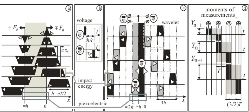
_{and at}x>0_{. Pulse of voltage}ϕ( )t _with du-ration τ <<F h c/ creates two normal displacement pulses (of mutually oppo-site polarity and of the length h) running to the left and to the right (see Figure 2(a)). Piezoelectric forces ±F# and F# of compression (tension) are

mu-tually balanced and need not mechanical support. Next we consider two piezoe-lectric layers

− < ≤ −

2 h x

h

_and

− < ≤

h x

0

_{excited by voltage pulses}ϕ( )t and ϕ( )t _{(Figure 2(b)) of the same duration but separated in time from each} other by the delay

h c

/

and with mutually opposite polarity. It is easy to see (Figure 2(c)) that at

x

≤ −

2 h

pulses of normal displacement created by voltage pulses (applied to above layers) are mutually compensated. But at x>0_these

pulses of normal displacement form the bipolar wavelet with duration

3 /

h c

and pause of duration

h c

/

between pulses. This wavelet is created also without any mechanical support [3].

If the impact duration (τ <<F T) is negligible, then we can write the wavelet

( )ξ

Ψ ₍ξ = −x ct_{, running to right) of single-direction radiation in the} follow-ing form: Ψ( ) { [ ] [ξ = I ξ −Iξ−(1/ 2) ]} { [T − Iξ−T] [−Iξ−(3 / 2) ]}T _{, where}

2 /

T

=

h c

_, I( ) 1ξ = _atξ>0_, I( ) 0ξ = _atξ≤0_{. Summarizing these}

wave-lets with amplitudes Yn_{and shifted with respect to each other by time distance}

2 /

T

=

h c

, we can form a sequence of hooked wave with duration

3 /

h c

_of each: Y0Ψ( )t Y+ Ψ −1 (t T)+ Ψ −Y2 ( 2 )t T + (Figure 2(d)). In this case we

(5)

[image:5.595.61.541.63.279.2]

Figure 2. Supportless flat impact. Formation of a normal displacement pulse (instant spatial distributions at different moments of time). Single-layer piezoelectric (a). Voltage excitation pulses ϕ( )t , ϕ( )t _{of a two-layer piezoelectric (b). Two-layer}

piezoelectric dynamics (c). Summarizing the wavelets in time at boundary x=0 (d).

the amplitude of the wavelet must be double, in order to provide, on average, the de-sired value of the normal displacement on the period

T

=

2 /

h c

_{. Thus, we obtain} the following expression (control algorithm) of the current amplitude Yn_{of the}

wavelet through via amplitude Yn−1_{of the previous and measured displacement} 1

( , n )

U⊗ R t− _{of the piston, as well as the required displacement}U•( , )R tn value

1 2[ ( , ) ( , ; , , ,...,1 0 1 2 1)]

n n n n n

Y Y= − + U• Rt −U⊗ Rt Y Y Y− Y− ,

(1) where tn=nT ,

n

=

0,1,2,...

The above-mentioned spreading of the imprints of

the blows (for compensation of which is necessary the impact pumping) is con-tained in the measured quantity U⊗( , ; , , ,...,R t Y Y Yn−1 0 1 2 Yn−1). Note that an

at-tempt to synthesize a desired value U•( , )R t using bipolar wavelets Ψ( )t means that the amplitude Yn of the wavelets is proportional to the integral of

the quantity U•( , )R tn −U⊗( ,Rtn−1). Thus, neither the measured displacement

( , )

U⊗ Rt _{nor the desired value}U•( , )R t should contain time-constant com-ponents. To maintain stability, it is necessary to exclude the constant component of the signals U⊗( , )Rt _andU•( , )R t , i.e. pass them through a non-distorting differential filter with a time scale τd>>λmax/c. Now we must note that slow

desired trajectory U•( , )R t of piston in time (with time scale τmax =λmax / 2c)

requires significant value of wavelet magnitude at some maximum amplitude

max

A of particle displacement in the waves to be damped. So the condition of linear flat impact becomes the following: (τmax/ )T Amax <<cτF <<cT<<L.

2.3. Measuring

(6)

V. V. Arabadzhi

[image:6.595.212.540.66.200.2]

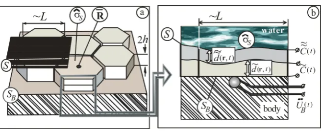
Figure 3. Tangential (a) and transverse (b) structure of active shell.

(between piezoelectric impacts) the current average piston (with the center in the point R∈S) area r∈σˆS⊂S particle displacement

( , ) B( , ) ( , ) ( , )

U⊗ R t U= R t U+  Rt U+  R t , where UB( , )Rt –slow displacement of

surface SB , where 1

ˆ

ˆ { ( , ), ( , )} ( ) { ( , ), ( , )} ( )

S S

U t U t d t d t d

σ

σ − σ

=

_∫



 _ _

 _R  _R _r _r _r _are

in-stant spatial average in the area r∈σˆ_S of the thicknesses d( , )rt , d t( , )r of the metallized layers of the piezoelectric. The smoothness of the distribution of displacements of the surface SB in space is guaranteed by the condition

min>>L

 , where max is maximum spatial scale of displacement distribution

on the surface SB). Therefore, UB( , )Rt can be used without spatial averaging

over the piston pad. Then we need to measure the instant capacitances C t( )

and C t( ) of the flat capacitors (dielectric layers) with varying thicknesses

~ ~

{ ( , ), ( , )}d t d t r  r = +h d{ ( , ), ( , )} r t d rt (where the variable components are rela-tively small, i.e. d~ <<h, d~ <<h) of the dielectric (piezoelectric) layers:

1 0

ˆ

{ ( ), ( )} ( ) ( ) /{ ( , ), ( , )}

S S

C t C t d d t d t

σ

ε ε − σ

∈

=

_∫



 _ _

 

r

r r r , where ε0—dielectric constant

of vacuum, ε—relative permittivity of piezoelectric. Now we write down the needed quantities { ( , ), ( , )}U Rt U Rt = −h C t C t[{ ( ), ( )}  −C0] /C0, where

0 S / ( 0 )

C =σ ε εh _{. These spatial averaging electric operations can be performed} almost instantaneously. Inertial accelerometer with output signal U tB( ) (i.e. the 2-nd derivative of normal displacement U tB( ) of body surface) is placed immediately under the center

R

of piston. In the end, we write down the re-maining component

0 0

ˆ

( , ) t ( )

B B

U Rt =

_{∫ ∫}

d LULξξ  η ηd , where Lˆ means 3-fold processing by differentiating chain with time scale τd >>λmax /c.

3. Scattering Suppression

Suppose that body’s radiation is already suppressed by the system described in Section 2. Further suppose that in area of compressible medium (with mass density ρ and sound speed c, identical with outer medium) delineated by surface S we know the particle displacement field U rI( , )t _{created by the} incident waves. Scattering field does not arise if we create on the outer surface of active shell the distribution U•( , )rt =n r U r( ) ( , )I t _{of normal displacements}

( , )

(7)

3.1. Incident Waves

Further we assume that incident wave field PI( , )rt = ΣnN=I1PIn( , )r t _{of pressure} represents the finite set of NI ≥1_{planar waves}PIn( , )rt = ΘIn[ ( , ) ]t− w rn c−1 , with vectors wn (wn =1) of propagation direction and profiles ΘIn( )ξ _with

leading edges: this means that there is a point ξn, for which the following

condi-tion is satisfied: ΘIn( ) 0ξ = at any ξ ξ< n, ΘIn( ) 0ξ ≠ at ξn< <ξ ξn+(λmin/ 4),

where λmin is the minimum length of the wave to be damped.

3.3. Spacing of Microphones

All the microphones are placed in points r r= •₍r•_{means the coordinate of} any microphone). In addition, all microphones are placed by pairs in points

•=

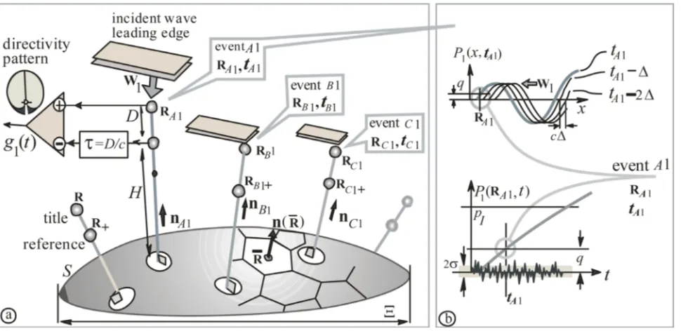
r R (farer to S_{and called “title microphone”) and}r R•= + (nearer to S and called “reference microphone”) on the normal n n R= ( )_{to a smooth convex} surface S with distance D between them (see nA1, nB1, nC1_{in Figure 4(a)). So}

vector R+−R is parallel to normal n n R= ( ) and R+= −R Dn R( ). Distance between reference microphone (in the point r R•= +) and surface S we will de-note H H= ( )R+ >>h D, . Points R presents the vertices of some convex po-lyhedron. Further, we will not designate microphones with specific numbers to simplify the presentation. At some initial moment, the leading edges of all the incident waves have not yet reached any title microphone. Note that all micro-phones should be insensitive to pressure fluctuations at a very high frequencies

2 /

π

T

≥

corresponding to the surface S_{flat impacts (Section 2).}

3.3. Arrival of 1-

st

_{Incident Wave}

Radiation of internal sources within surface SB is assumed suppressed by the

[image:7.595.60.545.461.697.2]

(8)

V. V. Arabadzhi

DOI: 10.4236/jamp.2018.611191 2310 Journal of Applied Mathematics and Physics means described in Section 2. All microphones are waiting for the first incident wave arrival from unknown direction w1 (output pressure signals of all

microphones are denoted by P1[ , ]r• t ). Leading edge of some plane incident wave (we will call this wave the 1-st incident wave with direction vector ) achieves some microphone spaced the in the point r R•= A1 at some moment

1 A

t t= _{. This is some space-time node (or event}_A_{1): module} P₁(RA₁, )t of

output signal of microphone spaced in the point r• =RA₁ sound pressure 1[ A1, ]

P R t crosses at the first time some level q from P1[RA1, ]t <q to

1[ A1, ]

P R t >q at the moment t t= A1. We notice a similar event B1 later on

some microphone with coordinate r R•= B1 at some moment t t= B1≥tA1:

module of pressure P1[RB1, ]t crosses at the first time some level q from

1[ B1, ]

P R t <q to P1[RB1, ]t >q_{at the moment}t t= B1. And the next similar

event C1 in the point r R•= C1 at some moment t t= C1≥tB1: module of

pressure P1[RC1, ]t crosses at the first time some level q from P1[RC1, ]t <q to 1[ C1, ]

P R t >q at the moment t t= C1. Assuming below the ratio pI >> >>q σ

(where pI_{is the characteristic amplitude of the pressure in the incident wave,}

and σ –the mean square deviation of background noise signal, see Figure 4(b)), we obtain the propagation vector w1=w1( 1, 1; 1)A B C _{of the 1-st incident wave}

from system of equations (RB1−R wA1) 1 =c t(B1−tA1)_and

1 1 1 1 1

(RB −R wA) =c t(B −tA). Usually incident wave is sufficiantly powerful

because one need to detect scattered wave at a large distance from the body. Now for stability of the active system we need to form signal of the incident wave pressure, insensitive (simplest spatial filtration) to waves scattered by the surface S due to possible violation of the condition uS( , )rt =n r U rS( ) ( , )I t . To

do this, we will form фa leading pair of microphones or a combination

1( ) ˆ 1[ A1, ] ˆ 1[ A1 , ]

g t =LP R t −LP R + t−τ of signals P1[RA1, ]t and P1[RA1+,t−τ] two microphones (in points RA1 (title microphone) and

1 1 ( 1)

A+= A −D A

R R n R (reference microphone) with cardioid directivity pattern having zero in the direction to the surface S (see Figure 4(a)). Here

τ =

D c

/

–delay, Lˆ–linear filter, undistorting signals at frequencies ωmin≤ ≤ω ωmax

( LPˆ I =PI ) and opaque for frequencies 0< <<ω ωmin , ω>2 /Tπ >>ωmax .

Under the condition D<<2 /π ωc max we obtain g t1( )= ∂ ∂τ( / ){t LP R tˆ 1[ A1, ]},

and for P1[RA1, ]t =PI1[RA1, ]t (1-st incident wave) we obtain

1

1 1

1[ 1, ] 1[ 1, ]1 [1 ( 1 1)] _C 1( ) t

I A C A A _t

P t ₌P t ₊

τ

− ₋ − g

ξ ξ

d

∫

R R n w (note that we have

1 1

(n wA ) 0< for any incident plane wave). Knowing the pressure field PI1 of

the first incident plane wave at a point RA1 at time t t> A1, we can determine

the pressure field at any point r (satisfying the condition (r R w− A1) 1>0) at

time t t> A1. In addition, we can determine the normal displacement uS( , )r t _of

the surface S under which the condition uS( , )rt =n r U rS( ) I1( , )t _{will be}

satisfied (the displacement field U rI1( , )t in the first incident plane wave in

infinite homogeneous compressible medium) and scattering will not arise. More precisely, we will establish a normal average over the area σˆS of the piston

(9)

1 1 1 1

( , ) ( , ) I[ A, ]

U_• Rt T+ =U_• R t +δP R t−α (2) (correcting it for a period of duration T, i.e. pressure-velocity-displacement), where δ1=( /T ρc)(w n R1 ( )), α =1 w R R1( − A1) /c. After inserting (2) into (1),

where t T t+ = n, the scattering does not occur, then the field of the first incident

wave PI1[ , ]r t passes without distortion through the region of space occupied by

the body and bounded by the surface S. And this means that the pressure field of the first incident wave PI2[ , ]r• t (for t t> C1) can be subtracted from the signals

of all microphones except for the leading pair (at points RA1 and RA1+) of the first incident wave. The sound pressure on the microphones at the points

1, 1

A A

•≠ +

r R R _{will now be denoted as} P₂[ , ]r• t =P₁[ , ]r• t P− I₁[RA₁,t−β₁], where

1 1( A1) /c

β =w r R_•− . Thus, we prepared the system for capturing a second plane incident wave, with respect to which we will assume that for the first points of contact of the leading edge with the microphones there will be points

1, 1

A A

•= ≠ +

r R R R _{of placement of the title microphones. The microphones at} the points r R R•≠ A1, A1+ became deaf (insensitive) to the first incident wave. Therefore, one can apply the logical procedure described above to the signals

2[ , ]

P r• t (three events A2 (tA2, RA2), B2 (tB2, RB2), C2 (tC2, RCA2)). And so

on. Below we give briefly a sequence of next functional steps.

3.4. Arrival of 2-

nd

Incident Wave

Event A2: t t= A2; r R•= A2; crossing P2 < ⇒q P2 >q. Event B2: t t= B2; 2

B

•=

r R ; crossing P2 < ⇒q P2 >q. Event C2: t t= C2; r R•= C2; crossing

2 2

P < ⇒q P >q_.

2 2 2 2 2

(RB −RA )w =c t(B −tA ), (RB2−RA2)w2 =c t(B2−tA2),

2= 2( 2, 2, 2)A B C

w w ,g t2( )=LPˆ 2[RA2, ]t −LPˆ 2[RA2+,t−τ],

2 ( /T c)( 2 ( ))

δ = ρ w n R , α =2 w R R2( − A2) /c,

2

1 1

2[ 2, ] 1[ 2, ]2 [1 ( 2 2)] _C 2( )

t

I A A C A _t

P t ₌P t ₊

τ

− ₋ − g

ξ ξ

d

∫

R R n w , β2=w r R2( •− A2) /c,

1 1 1 1 2 2 2 2

( , ) ( , ) I[ A, ] I [ A , ]

U_• R t T+ =U_• R t +δ P R t−α +δ P R t−α ,

3[ , ] 3[ , ] I1[ A1, 1] I2[ A2, 2]

P r_• t =P r_• t P− R t−β −P R t−β , for n

1, 1, 2, 2

A A A A

•≠ + +

r R R R R .

3.5. Arrival of 3-

rd

_{Incident Wave}

Event A3: t t= A3; r R•= A3; crossing P3 < ⇒q P3 >q. Event B3: t t= B3; 3

B

•=

r R ; crossing P3 < ⇒q P3 >q. Event C3: t t= C3; r R•= C3; crossing

3 3

P < ⇒q P >q.

3 3 3 3 3

(RB −R wA ) =c t(B −tA ),

3 3 3 3 3 3 3

(RB −R wA ) =c t(B −tA )⇒w =w ( 3, 3, 3)A B C ,

3( ) ˆ 3[ A3, ] ˆ 3[ A3 , ]

g t =LP R t −LP R + t−τ , δ3=( /T ρc)(w n R3 ( )),

3 3( A3) /c

α =w R R− ,

3

1 1

3[ 3, ] 3[ 3, ]3 [1 ( 3 3)] 3( )

C t

I A A C A _t

P t ₌P t ₊

τ

− ₋ − g

ξ ξ

d

∫

R R n w ,

3 3( A3) /c

β =w r R_•− ,

1 1 1 1 2 2 2 2 3 3 3 3

( , ) ( , ) I[ A, ] I [ A , ] I [ A, ]

(10)

V. V. Arabadzhi

4[ , ] 3[ , ] I1[ A1, 1] I2[ A2, 2] I3[ A3, 3]

P r_• t =P r_• t P− R t−β −P R t−β −P R t−β , for

1, 1, 2, 2 , 3, 3

A A A A A A

•≠ + + +

r R R R R R R .

4. Conclusion

The main results of this work are the following: 1) transparent supportless un-idirectional sources of acoustical wavelets (Section 2), 2) causal sequence of op-erations to reconcile the normal displacements of the protected surface with the incident waves (Section 3). The presented results are a consequence of the problem formulation with initial conditions and could not be obtained in the widespread stationary monochromatic mathematical model of the problem with complex am-plitudes (magnitude A, frequency ω, phase ϕ, i.e. Aexp[ (i tω ϕ+ )]_{) of the} fields (like in [2] for instance). The monochromatic representation leaves out of view some important situations, such as spatio-temporal labyrinths, where the control algorithm (like “Maxwell’s demon”) operates extremely quickly on the spatial microscales, and this leads to macroscopic results for long slow waves [3].

Conflicts of Interest

The authors declare no conflicts of interest regarding the publication of this pa-per.

References

[1] Bi, Y.F., Jia, H., Sun, Z.Y., Yang, Y.Z., Zhao, H. and Yang, J. (2018) Experimental Demonstration of Three-Dimensional Broadband Underwater Acoustic Carpet Cloak. Appl. Phys. Lett., 112. https://doi.org/10.1063/1.5026199

[2] Cummer, S.A., Popa, B.I., Schurig, D., Smith, D.R., Pendry, J., Rahm, M. and Starr, A. (2008) Scattering Theory Derivation 3D Acoustic Cloacking Shell. Physical Re-view Letters, 100.