Towards autonomous motion of the PIRATE through closed pipe structures The Sensing System

(1)

TOWARDS AUTONOMOUS MOTION OF THE

PIRATE THROUGH CLOSED PIPE STRUCTURES

D.M.G. (Dinah) Kleiboer

MSC ASSIGNMENT

Committee: prof. dr. ir. G.J.M. Krijnen N. Botteghi, MSc dr. ir. E. Dertien dr. ir. R.G.K.M. Aarts

December,2019

052RaM2019

(2)

Master Systems & Control

Robotics & Mechatronics

Master Thesis:

Towards autonomous motion of the

PIRATE through closed pipe structures.

The Sensing System

Author:

Dinah M G Kleiboer

Student number: 1449559

Head Graduation Supervisor: Prof.Dr.ir. G.J.M. Krijnen Daily Supervisor: N. Botteghi MSc

UT Supervisor: Dr.ir. E.C. Dertien External Supervisor: Dr.ir. R.G.K.M. Aarts

(3)

Preliminary

1.1 Introduction

In recent years the use of autonomous robots for tedious tasks has grown, especially for the inspection and maintenance of places that are hard to reach and/or dangerous for humans. Complex industrial pipe networks are such a place, as these often transport dangerous chem-icals or gasses. Failure to inspect and replace damaged pipelines in a timely manner may result in catastrophic accidents. The inspection tasks include localization of defects and de-formations, and the verification of the pipe its wall thickness. These are currently only able to be performed manually from the outside [1]. The pipes, however, are often unreachable or may be covered with isolation materials, making inspection very difficult, time-consuming and costly. Therefore, an autonomous driving system is being developed at RAM to facilitate the inspection of these. The key requirements for this Pipe Inspection Robot for AuTonomous Exploration (PIRATE) are its size limit and its maneuverability, i.e. it should be able to navigate on its own through pipe structures with diameters ranging from 57 mm to 125 mm, and various bends such as 90°elbows and T-junctions [2]. Since its initial design, the PIRATE has undergone several hardware and software design changes and improvements [3], [4], [5], [6]. Some details on the current design and capabilities of the PIRATE are explained next.

Figure 1.1: Design model of the PIRATE prototype II [6].

1.2 PIRATE Background

(6)

Master Thesis Preliminary

both physical configuration and computational load [7]. Reiling researched and designed a structured light sensor that in theory can be made small enough for autonomous navigation through 57 mm diameter pipes and inspection of these. His work was somewhat resumed by van der Meer who used this sensor to create 3D reconstructions of inner pipe segments for fast obstacle and junction detection. The working principle of this sensing module is explained further in section 2.1.3.

(a) The sensor camera system and control boards. (b) The projected light inside a pipe.

Figure 1.2: The structured light sensor previously designed for the PIRATE [8].

Additional steps toward PIRATE autonomy were taken by Geerlings [6], through the implementation of sequences of motion primitives in the software. As the name states, these sequences hold a certain order of basic motion commands for specific tasks, such as ‘Take a turn’. In experiments these motion primitive sequences are triggered by an external overhead camera and markers, see appendix A for a short explanation [6]. Full autonomy, however, remains to be accomplished.

1.3 Problem Statement

For efficient inspection of industrial pipelines, operating the PIRATE has to be straightfor-ward allowing the operator to focus on examining the condition of the pipe. Therefore, some level of autonomy is required, which means that the PIRATE should take certain decisions on its own. Specifically focusing on navigational autonomy through complex pipe structures, the sensing system of the PIRATE needs to be improved to properly detect and identify junctions and obstacles in time to take a turn or stop.

The aim of this project is to research and develop an improved on-board sensing system the PIRATE can use for autonomous navigation through varying pipe structures. For this, a different approach is taken from the previously mentioned methods. The corresponding research question and supporting sub-questions are as follows

How can the PIRATE efficiently detect and identify complex closed pipe structures, for autonomous navigation through these, using an on-board sensing system?

I Is a 2D LiDAR sensor sufficient to recognize a mitre bend in a closed pipe structure?

(7)

Master Thesis Preliminary

To properly answer these questions, the research focuses on clarification of the abilities and possible solutions for the sensing system. Clarification points of interest are, for example, ‘What type of pipe structures may be encountered exactly?’ and ‘How much autonomy should the PIRATE actually have?’. The possibilities for sensing solutions are gathered from research on previously developed systems used for similar operations. Once the research is concluded the development process focuses on the hardware and software of the sensing system used for obstacle and junction detection. Some key requirements are to obtain a wide Field of View (FoV) and accurate sensor data, that is easy to interpret with the detection algorithm. The detection algorithm in its turn has to analyse the measurements in a computationally efficient manner to quickly obtain information that can be used for navigation in pipelines. The effectiveness of this system will then also be compared to the previous sensing system, by E. Dertien [7], to determine if it indeed provides a better solution for the PIRATE.

1.4 Outline

(8)

“The only true wisdom is in knowing you know nothing.”

— Socrates

Background

2.1 State of the Art

In this chapter we dive into the works of previously developed (autonomous) pipe inspection systems and look at how autonomy can be defined clearly. Then a deeper dive is taken into the workings of the two most promising hardware solutions.

2.1.1 Pipe Inspection Systems

Around the globe, companies have the problem of conducting proper pipe-inspections. To solve these problems scientists are developing (semi-)autonomous robots that carry out the inspections of various pipe structures. One of the challenges in creating such autonomous systems is the implementation of a sensing system that is small enough yet capable to detect and distinguish different pipe junctions. In the autonomous robots FAMPER and MAKRO, sound waves are used to detect bends and obstacles in front of the robot utilizing sonar and ultrasound sensors, respectively [10], [11].

Figure 2.1: The AIRo2.1 with an LED and camera sensing module [12].

Figure 2.2: The MRINSPECT VI Sensing module [13].

Many self-driving systems make use of vision-based obstacle detection, either by Time-of-Flight (ToF) light sensors or in the form of cameras combined with image processing. The AIRo 2.1, in figure 2.1, and MRINSPECT make use of lights and a camera for shadow detec-tion at juncdetec-tions [12], [14]. For MRINSPECT V Lee et al. implemented image recognidetec-tion of a line laser beam projection to detect pipe features, as is done in figure 2.3. This method is based on the fact that different types of junctions have different patterns, as in figure 2.3a1. Even though junctions can be detected very well, the method shows errors in differentiating between T-junctions and miter bends and suffers from noise on the image. For the MRIN-SPECT VI the researchers, therefore, decided to add PSD (Position Sensitive Device) sensors to measure the distance to an obstacle in front of the robot and the radial distance to the side-wall or junctions, placed as can be seen in figure 2.2. This method showed to be better in differentiating bends and also required a lower computation load [13]. A similar sensing method is also seen in PIKo which utilizes a 3D ToF camera for depth perception [15]. The exact detection method used is based on that of Thieleman et. al. in [16]. Their idea uses a virtual projection of a cylinder or cone along the pipe walls, the points that are not on the

(9)

Master Thesis Background

surface of the cylinder are collected in blobs. These blobs are then used to identify the pipe properties based on their shape and size.

In unknown networks of small pipelines with little variation in characteristics, it is difficult for some sensors to detect landmarks without using high computation loads. Therefore, researchers at the University of Manchester came up with the idea of using mechanical feelers in front of their robot, FURO, to detect the direction and radius of upcoming junctions [17]. A drawback of this method is that the junction is detected relatively late, depending on the length of the feelers. This poses restrictions on the maximum speed of the robot, its size and the diameter of the pipe in which it can be used.

(a) Characteristic image of a straight pipe (L), an Elbow (C) and a T-junction (R)1_.

(b) The image processing procedure.

Figure 2.3: Line laser beam projection used for the MRINSPECT V [14].

2.1.2 Robot Autonomy

(10)

[image:10.612.115.490.331.696.2]

Figure 2.4: Flow chart, of the framework by Beer et. al., to determine robot autonomy [18].

Figure 2.5: Table of the autonomy level proposed by Beer et. al. [18].

(11)

2.1.3 The Sensory System

As stated in the previous section, for any autonomous system a good sensing part is required to detect surrounding obstacles. Looking at one of the most complex ‘autonomous systems’ known, the human body uses (in the optimal case) three sensing methods; namely vision (light detection), hearing and feeling, with the sensory system to process the observations. Great technological advances made it possible to, a certain extent, implement these sensing methods in robots. As has been done for the various pipe-inspection robots mentioned in section 2.1.1. Research on these inspection robots show that sound detection is not optimal in closed pipe structures. The same holds for mechanical feelers, which would also make the PIRATE design more complex. Thus, the best solution is some type of vision-based sensing module, such as a camera, a light-based depth sensor or a combination of these. These are, therefore, shortly analyzed below.

Camera

Cameras provide visual data that is relatively easy to interpret by humans. It is, therefore, not surprising that they are implemented in robotic pipe inspection systems, such as the AIRo2.1, MRINSPECT and PIKo mentioned in section 2.1.1. For navigation, it is important to have some sense of depth perception, which can be obtained from binocular or stereo vision. These utilize at least two cameras to create 3D reconstructions from the separate camera images of an object. In the absence of clearly identifiable objects, this method may not be optimal. Therefore, the use of structured light with a single camera for detection is considered a better alternative for inner pipe navigation, as used for the MRINSPECT [14] and the previously designed PIRATE sensor [8], for example. The structured light can be projected in different shapes and sizes, such as cones, lines or dotted configurations, as long as the orientation and dimensions of the projection are known. Both methods work on the same principle of optical triangulation, of which the general idea is depicted in figure B.3 in the appendix, to obtain distance data for 3D reconstructions. Image processing is then required to extract the properties of interest. Note that details on the exact working principles and procedures of these methods are left to the reader.

(12)

LiDAR

Recent developments in self-driving vehicles have used Light Detection and Ranging (LiDAR) with great success to detect the immediate surrounding. LiDAR is a type of Time-of-Flight (ToF) sensor that emits light or laser pulses onto the surface of nearby objects and measures the time it takes for this light to be reflected to the detector. The distance (d) to the object is determined from the arrival time (t) with equation (2.1), where c is the speed of light and

nis the refractive index [19]. A great benefit of LiDAR is the fact that it provides numerical data, so no extra computation is necessary to determine the distance to objects.

d= c·t

2·n (2.1)

There are different types of LiDAR sensors, the 1D sensor is the most common and inex-pensive. As the name depicts, it measures the distance to a point using a single laser beam. For 2D and 3D data, many sensors simply rotate a 1D LiDAR. The technology is still under development and solid-state 2D and 3D sensors are upcoming. Such solid-state sensors are more robust and have faster measurement rates, as the sensors generally send out an array of laser points.

Figure 2.6: Example point cloud of a cylindrical object, with the RGB points visualized with respect to the coordinate system originated in the center [20].

Point Clouds

(13)

be obtained if the measurement frequency, of the complete environment of interest, is faster than the driving velocity. If a 1D LiDAR is used to obtain a 3D point cloud, for example, it is necessary to rotate the sensor in every single direction, for a full Field of View, before the robot moves to the next position. This to avoid not scanned areas, which will result in empty parts in the point cloud and inconsistent data that may be identified wrong in future processing.

2.2 Theoretical Background

In this chapter, the theoretical background used for the detection and identification of different pipe structures with the detection algorithms is explained. Furthermore, the exact pipe structures that may be encountered and the methods used to correctly identify these are discussed.

2.2.1 Pipe Structures

Gasses and chemicals have to be transported to various locations on an industrial plant or even throughout the country. The pipe networks used for this are far from simple straight pipelines, different pipe connections are used instead to change direction and sometimes even to adjust the pressure inside. For this study, it is considered that pipe fittings can be categorized into three main types: reducers, bends and junctions. The categorization is based upon the motion choices that have to be made when such a section in a pipe is encountered by the PIRATE. The properties of these types are shortly described below.

Type 1: Reducers

Reducers can be recognized as a straight pipe section with a change in diameter. Figure 2.7 shows that this type also includes pipe closures or obstacles, which can simply be seen as a diameter reduction to 0 mm. When this type is encountered the PIRATE likely has to change its clamping angles to the new diameter. If this diameter is smaller than the minimum of 57 mm, then the PIRATE must stop and go back.

Figure 2.7: Pipe segments to change radius or close a pipe [21].

Type 2: Bends

(14)

Figure 2.8: Pipe bends of various angles [21].

Type 3: Junctions

This type consists of the more complex structures that come in many different forms. Several types of junctions include, but are not limited to, T-, Y- and cross junctions, as depicted in figure 2.9. At a junction, there are usually multiple navigational options the PIRATE can take. Here, it is thus very important to first identify the number of options and the direction in which they are in. Since the diameter may also change at a junction, this also needs to be determined as well as the angle of the turn to be taken.

Figure 2.9: Different types of pipe junctions [21].

2.2.2 Measurement Transforms

(15)

changes. Considering a LiDAR sensor rotates on an axis parallel to the pipe, i.e. they-axis in figure 2.10, the radius can easily be calculated. Figure 2.11 provides a good reference for this calculation. Here the center of the pipe is taken as the origin and thex- andz-axis are the distances to the pipe wall. It is assumed that the distance (xP) to the positionP of the

sensor along thex-axis is known. This may be obtained from the angle encoder on the front module of the PIRATE, for example. The sensor measurements give the distance (d) from

P toSA and SB, which is equal to thex-coordinate as calculated for the 2D case. Since the

angleα is also known from the motor that rotates the sensor, the radius r can be calculated with the following equations, which are the same for bothrA and rB.

xs =d cos(α) (2.2a)

zs =d sin(α) (2.2b)

r =

q

z_S2+ (x_P+x_S)2 _(2.2c)

[image:15.612.97.533.258.538.2]

Figure 2.10: Top view of a 2D scanner inside a pipe.

Figure 2.11: Cross-section of a Pipe with a 2D scanner inP to cal-culate the radii (r).

2.2.3 Ellipse Fitting

The general equation of conics is of the form given in equation (2.3). For this equation to specifically represent an ellipse the condition in equation (2.4) has to be satisfied. Note that a circle is just an ellipse of which the length of the semi-axis is equal.

ax2+bxy+cy2+dx+ey+f = 0 (2.3)

b2−4ac <0 (2.4)

(16)

the set of parameters (a) that minimize the sum of squared algebraic distances between the points, as follows

min

a N

X

i=1

F(xi, yi)2 = min a

N

X

i=1

(xi·a)2= min

a kDak

2 _(2.5)

where

a= [a, b, c, d, e, f]| xi= [xi2, xiyi, yi2, xi, yi,1]

D=         x1 .. . xi .. . xN         (2.6)

representing the general (equation (2.3)) in matrix-vector form. Note that the Design matrix D has sizeN×6.

To simplify the calculation of an ellipse specific equation the condition in equation (2.4) is transformed to the equality condition, equation (2.7), obtained by rewriting and proper scaling [23].

4ac−b2 = 1 (2.7)

Using the Lagrange multiplier (λ) method the system of equations is reduced and solved for ausing

Sa=λCa

a|Ca= 1 (2.8)

where theConstraint matrixCrepresents equation (2.7) and theScatter matrixS=D|D. The improved method of R. Halir and J. Flusser [22], focuses on solving the decomposed form of this system of equations. Herein the decomposed Design matrix D = (D1|D2) with D1

and D2 (see equation (2.9)) consisting of its quadratic and linear parts, respectively.

D1 =

       

x2₁ x₁y₁ y₁2

..

. ... ...

x2_i x_iy_i y_i2

..

. ... ...

x2

N xNyN yN2

       

D2=

       

x1 y1 1

..

. ... ...

xi yi 1 ..

. ... ...

xN yN 1

(17)

The resulting Scatter matrix, Constraint matrix and the vector of parameters to solve are

S=

S₁ S₂ S|₂ S₃

with

S1=D|1D1

S2=D|1D2

S3=D|2D2

(2.10)

C=

C1 0

0 0

with C1=





0 0 2

0 −1 0

2 0 0

  (2.11) a= a1 a2

with a1 =

  a b c 

and a2 =

  e f g   (2.12)

By completely rewriting equation (2.8) using the above matrices the final set of equations to be solved becomes

Ma1 =λa1 (2.13)

M=C−₁1(S₁−S₂S−₃1S|₂) (2.14)

a|₁C₁a₁ = 1 (2.15)

a₂ =−S−₃1S|₂a₁ (2.16)

From these the final solution is found by calculating the eigenvectora1, of thereduced

(18)

“Make it simple, but significant.”

— Don Draper

Design Analysis

3.1 Requirements & Specifications

3.1.1 PIRATE Autonomy

Of course, a fully autonomous inspection system is the ultimate goal for the PIRATE project, but for several technical reasons this will remain a big challenge. Therefore, a certain degree of system autonomy has to be assigned to the PIRATE, at least for the time being. Doing this will aid in the further development of the PIRATE and the design choices to be made.

To determine the desired level of autonomy the framework of Beer et. al., described in section 2.1.2, is used. Following the guidelines in figure 2.4, it is considered that currently the task the robot is to perform is driving through varying industrial pipe structures without bumping into obstacles. Note that the action of inspecting the pipe for defects is omitted during this assignment. The aspects of the task that the PIRATE should perform include: detecting and identifying a turn, then driving towards the turn and performing the correct sequence of motions to manoeuvre the turn and continue driving. In terms of the primitives, sense, plan and act stated in section 2.1.2, the PIRATE must hold a high level of the sensing and acting ability. The actual planning of ‘where to go’ is mostly left to the human operator. From these specifications the PIRATE autonomy can be categorized using the defined levels of robot autonomy in figure 2.5. The aim is to reach the ‘Decision Support’ level of autonomy, which is defined as“Both the human and robot sense the environment and generate a task plan. However, the human chooses the task plan and commands the robot to implement actions.”

[18].

As mentioned in section 1.2, motion primitives are already successfully implemented, enabling the PIRATE to perform the right motions to take a turn on its own when instructed. Thus, a sufficient level of autonomy to act is already established. The goal of this assignment is to also reach a higher level of autonomy in the sensing capabilities of the PIRATE, which will aid in motion planning and straight forward operation of it.

3.1.2 System Requirements

The system requirements are the minimum set of abilities the PIRATE is expected to have for the sensing system under development. The main goal of this project is to obtain an on-board sensing system for the detection and identification of various pipe structures to reach the previously mentioned level of autonomy in the PIRATE. Based on this the requirements are determined and listed below following the MoSCoW method, which prioritizes these according to the Must, Should, Could and Won’t haves (MoSCoW).

Must

• The system must be able to detect and identify 90°miter bends.

• The sensor must be small enough to fit in the front module of the PIRATE, which has a diameter of 45 mm.

(19)

Master Thesis Design Analysis

trigger the motion primitives for the PIRATE to drive autonomously through a pipe structure in a horizontal plane.

• The algorithm must be able to accurately determine the distance to, and direction of obstacles and bends. For the distance the preferred accuracy is 2 cm and for the direction this is 5°.

Should

• The sensor should properly operate in all pipe diameters specified for PIRATE opera-tion, i.e. pipes with an inner-diameter between 57 mm and 125 mm.

• The system should be able to detect long and short bends of different angles, T-junctions, Y-branches and diameter changes in the pipe. These may occur in any direction of the pipe regardless of the orientation of the PIRATE.

• The detection algorithm should be able to properly distinguish and identify these com-plex pipe structures, following the categorization in section 2.2.1. The identification should provide pipe properties, such as the diameter and angle, that can be used for autonomous motion. The preferred accuracy with which these should be determined is also 2 cm for the size and 5° for the angle.

• The system should have fast computing/processing time to analyze the measured data and determine the type in time to take a turn.

Could

• A minimum 180°FoV of the sensor in both horizontal and vertical direction is preferred. This can be used to create a 3D point cloud and/or map of the structure.

• The detection of obstacles and junctions in the back of the PIRATE could also enable backward driving.

• The system could include a camera and LEDs for live image feedback to the operator and improved junction detection.

Won’t

• Other pipe inspection tools, such as ultrasound sensors, will not be included yet.

3.2 The PIRATE’s Sensory System

3.2.1 Hardware Design

(20)

considered to expand the research to other sensor types and compare the results. Generally, LiDAR does not require any calibration and can easily be integrated in the system. Off the shelf LiDAR sensors come in many shapes and sizes, mostly with measurement ranges from 0.1 m to 20 m. Depending on the type (1D, 2D or 3D) and the specifications, the price varies significantly. As the use of LiDAR for PIRATE navigation first has to be proven, the price should be kept at a minimum. Several off the shelf sensors, listed in table C.2 in appendix C, are considered for this project. Mostly due to size requirements some trade-offs are made between the range and a large Field of View (FoV). Therefore, the final choice for the sensor to integrate on the PIRATE is the ‘Small LS02 Solid State LIDAR’ by LeiShen Intelligent System [24]. For proper testing of the detection algorithm and to prove its performance in small diameter pipes, however, a better sensor is acquired. The ‘YDLidar X4’ has an ideal 360° FoV with 0.5° angle resolution, which can both be adapted in the software [25]. The specifications of both sensors are listed in table 3.1.

Table 3.1: Specifications of the ‘LS02 Solid State Lidar’ and the ‘YDLidar X4’ as provided by [24] & [25], respectively.

Specifications LS02 Lidar YDLidar Unit

Detection Range 0.1 - 4 0.12 - >10 m

Detection Accuracy <0.5 (for range <2 m) <3 % of distance mm

Scanning Angle 86 0–360 °

Angle Resolution 1 0.48–0.52 °

Scan Frequency 10 6–12 Hz

Volume 45×37×40 101×65×39 mm3

3.2.2 Software Design

Assumptions

Some important assumptions that are made during the design of the detection algorithms include the following.

i The PIRATE is perfectly clamped in the center of the pipe.

This is necessary to obtain the exact pipe diameter from the clamping angles.

ii Only pipe bends and junctions with a maximum angle of 90°, clockwise with respect to the centerline1 of the pipe, will be encountered. Long bends with an angle smaller than 30° will be considered as straight sections.

iii The LiDAR scanner is positioned with the front parallel to the centerline of the pipe, unless the exact angle with respect to the centerline is known. This is required for proper transformation from the distance measurements to Cartesian and polar coordinates.

iv Upcoming bends and junctions can be detected and identified from the outline that is formed on the wall of the straight pipe section (see figure B.4 for a clear representa-tion). To calculate the properties of this upcoming section the outline is assumed to be elliptical.

1

(21)

Detection algorithm for planar measurements

To determine whether a junction can indeed be detected or not, in C++ a detection algorithm is established that uses 2D LiDAR scans, i.e. distance measurements in a (horizontal) plane configuration. Because these measurements are taken at different angles originating from the origin, as in figure 2.10, a transformation to Cartesian coordinates in the same measurement plane is done first. The points are then divided into ‘left-’ and ‘right-side’ arrays, with the ‘left-side’ containing the points of negativex-coordinate values and vice versa. The idea of the algorithm is to calculate the average diameter of the pipe (dLidar) from these (x, y) points and

compare this to the known pipe diameter (dClamped), obtained from the PIRATE encoders

while clamped. Once a significant change in diameter, i.e. diameter±5 mm, is detected the algorithm loops through another calculation to determine if an obstruction, bend or junction is reached. The algorithm is summarized in algorithm 1 with steps A to D, the pseudo-code also shows the general outline of thegapDetection() function.

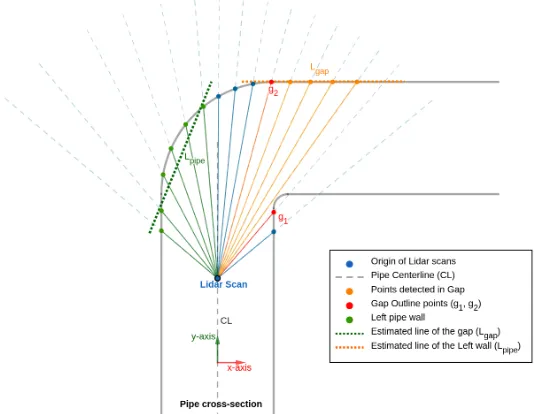
[image:21.612.158.425.512.719.2]

In the gapDetection() function, a bend or junction is detected as a ‘gap’ on either side of the pipe. Such a gap is identified by a minimum difference, equal to the minimum diameter the PIRATE can enter (57 mm), between the y-coordinates of consecutive points. This can be done as long as assumptionii holds. Then, all the points inside the gap are collected to determine the angle of the bend or junction. In the case of a bend, the slope of the closed side is also estimated to get an idea of the sharpness of the turn. By applying linear regression to each collection of points, the equation of a line through these can be estimated. The slope of this line is considered to be equal to the absolute angle of the gap or pipe being calculated. When a gap is detected, the y-coordinate of the points on the pipe wall, one right before and one after the gap, give the size of this gap. The distance to the center between these two points, is considered the distance to the entrance of the bend or junction. A visual representation, figure 3.1, provides a clear indication of this process. When no gaps are detected the distance to a possible obstruction is returned. If this distance is considered infinite, the upcoming pipe section is most likely a reducer of which the new diameter is returned.

(22)

Algorithm 1:General outline of the procedure for 2D detection. Data: ROS Topics of Lidar and other sensor measurements Result: Pipe properties

whileSubscribing to topics OK do read current

A. Transform, sort and temporarily store measurement data B. Calculate pipe diameter (d) and check difference

if dLidar==dclamped±errorthen

Keep going straight! else

Pipe structure detected! Diameter changes == true end

C. if Diameter changes then

[properties L] = gapDetection(Left side data)

[properties R] = gapDetection(Right side data)

else

Do nothing end

D. Output the total number of gaps detected and the calculated properties of each. end

FunctiongapDetection(data):

if ∆y-data ≥dminimum and x-data > dclamped₂ then

Gap detected! number of Gaps +1 end

if Gap detected then Determine:

gap Size = Max. distance between y-points on pipe wall gap Entrance= Distance to center between these y-points gap Angle= Slope of the points detected inside the gap else

Determine:

pipe Angle= Slope of the points detected on the pipe wall end

return number of Gaps,gap Size,gap Entrance,gap Angle,pipe Angle

End Function

Detection algorithm for 3D measurements

(23)

PIRATE. This is done to obtain symmetric measurements along the pipe wall, from which the diameter can be calculated easily. This rotation method also provides continuous ‘vision’ in front of the PIRATE. Note that with this method, assumptioniiialso remains valid during the complete rotation. In order to get good and consistent data, it is decided early on in the design process to rotate the sensor via position control. Which simply means that, instead of rotating the sensor at a constant velocity, it is set to a new angular position after all data points are obtained. The command to rotate to the next position and the increment with which this has to occur, are also send from the detection algorithm. This part of the process is not described further, instead the focus is set on the exact method used for junction detection in all directions. The 3D detection algorithm is, simply put, an advanced extension of the 2D detection algorithm described previously. The general working process for 3D detection of complex pipe structures is outlined in algorithm 2. For the calculations in this algorithm the LiDAR measurements are again transformed to Cartesian coordinates in the sensor plane first. With these coordinates and the angle of the servo motor, used to rotate the sensor, the radius of each point is calculated, using the method described in section 2.2.2. Once the average of these radii is significantly different from the known radius, for multiple angular positions, a non-straight pipe structure is said to be detected. The next step, step C in algorithm 2, is to determine the type of structure, as classified in section 2.2.1, this to avoid any unnecessary calculations. The method used to identify the structures is inspired by the one used for the PIKo [15] as presented by Thieleman et. al. in [16], which uses categorized measurements to track pipeline features. So instead of generating and saving the entire point cloud of measurements, only the points of interest are saved during each full scan of the pipe2. These points are collected, based on their radius, into an array of one of three categories: inliers, outliers or outline. The inliers are the points that have a radius smaller than that of the pipe. The outliers are the points with a radius larger than the pipe. And the outline holds the points around the outliers but on the pipe wall, as to portray the outline of a junction (see figure B.4 for an illustration). Note that due to the sensor accuracy some margin of error is included for this categorization. The properties of each array are then used, in step C.2, to determine the type of structure encountered by the PIRATE and to calculate the properties of these. For example, if there are no outline points, so the outline array is empty, the section is of type 1 and the inliers or outliers can be used to calculate the new pipe diameter in step C.3. In the case of type 2 or 3 and with assumption iv, each outline is used to estimate a circle or ellipse with the procedure described in section 2.2.3. The properties of the ellipse, i.e. the length and angle of the major and minor axis, are then used to determine the size and direction of the bend or junction. The y-coordinate of the center of the ellipse is considered to be the distance to the entrance of the upcoming structure. In the case of a junction (Type 3 or 4) there are usually multiple options the PIRATE can take, the properties of these are all calculated and output for the user to make a decision. When the algorithm runs successfully through these steps the possible options are displayed on screen and the result consists of a single value for the following properties:

• Distance - The distance to the center of the detected type of pipe section.

• Diameter - The diameter of the upcoming pipe section.

• Angle & Direction - The 3D angle of the turn the PIRATE has to take.

(24)

Once a choice is made which option the PIRATE should take, these calculated property values can be used in the motion sequence algorithm.

Algorithm 2:General outline of the procedure for 3D detection.

Data: ROS Topics of Lidar, rotation servo and other sensor measurements Result: Pipe properties

whileSubscribing to topics OK do

A. Transform, sort and temporarily store measurement data.

B. Calculate pipe radii (r) of each area (I, II) and compare to diameter (dclamped)

if rLidarI,II == dclamped

2 ±errorthen

No change in Area I,II else

Possible pipe structure detected! Radius changes == true

end

C. if Radius changes and new rotation starts then

1. Transform 2D to 3D data and Store points of interest in one of the following:

Inliers ←points with r < dclamped

2 −error

Outliers←points withr > dclamped

2 + error

Outline←points withr = dclamped

2 ±error

2. if Full 180° rotation is complete then Analyse data to determine section type:

if No Outlinethen returnType 1

else if 1 Outlineand Inliersthen return Type 2

else if multiple Outlineand Inliers then returnType 3

else return Type 4

end

3. Determine pipe properties based on Type: switch Type do

caseType 1 doCalculate reduction properties return diameter,distance

caseType 2 doEstimate ellipse fromOutline and calculate bend properties return distance,diameter,direction andangle

caseType 3, Type 4 do

Estimate ellipse and calculate properties for each Outline. if Type 4then Extra option to keep going straight.

return number of Options and distance,diameter,direction and anglefor each option

(25)

“Design is not just what it looks like and feels like. Design is how it works.”

— Steve Jobs

Experiment Design

4.1 Experiments

Whether the designed algorithm works or not depends on its performance during several tests, including computer simulated and practical tests. The simulations are done first, to aid in bug fixing and to avoid unwanted issues during practical tests. The practical tests are then performed to analyse if similar results can be obtained and to determine if the designed system is a good solution to aid in PIRATE autonomy. The methods and tools used for these experiments are described in this chapter. Table 4.1 provides a quick overview of the experiments that are done.

Table 4.1: Experiments done to analyse the performance of the detection algorithms. Note: α = angle of the bend, d= diameter of the pipe.

Test Reductions Bends Junctions

Simulation 2D x α: 90°

d: 6 cm and 10 cm x

Simulation 3D d: 45 % reduction α: 45° & 90°

d: 10 cm

X-junction

d: 10 cm

Practical setup 2D x α: 45° & 90°

d: 11.8 cm

T-& Y-Junction

d: 11.8 cm

Practical setup 3D x α: 90°

d: 20 cm x

PIRATE (2D ) x x x

4.2 Simulations

(26)

Master Thesis Experiment Design

Apart from a simulation done to check the performance of the ‘LS02 Solid State 2D LIDAR’ in small diameter pipes, several simulations are run specifically to determine the accuracy, reliability and limits of the 2D detection algorithm. The results of these should provide sufficient knowledge to answer sub-research question 1. Therefore, these tests are run in a 3D simulated CAD model of a (90°) mitre bend pipe structure. To determine the accuracy and reliability of the algorithm, the first test is executed several times for accumulation of multiple data sets. This test is simply done by translating the sensor block, with constant velocity along the pipe its centerline, toward the bend. To determine the limits of the system, regardless of the sensor specifications, the 2D detection algorithm is run for several misaligned positions of the sensor block. These misaligned positions consist of rotating and translating the sensor block away from the forward facing position along the pipe its centerline. Next, the ability to detect and identify pipe structures in different directions also has to be confirmed. This is done with the 3D detection algorithm and a rotating 2D LiDAR. This algorithm works best when enough points along the full pipe circumference are detected. Therefore, as proposed in section 3.2.2, the sensor is rotated about an axis parallel to the driving direction. Then the algorithm is run multiple times at different positions of the sensor block along the centerline of the simulated pipe structure. This to obtain enough data points, to check the output of the algorithm at each position and see how this changes when approaching the upcoming structure. The simulations for these tests include 3D CAD pipe structures of each type mentioned in section 2.2.1.

Figure 4.1: Example of the environment for the simulated tests.

Table 4.2: Specifications of the ‘ideal Lidar’ used in simulations.

Item Value Unit

Detection range 0.1–200 cm

Range resolution 0.1 cm

Field of View 180 °

Angle resolution 0.5–1 °

4.3 Practical Tests

(27)

de-Master Thesis Experiment Design

tected on either side of the pipe wall of small diameter pipes (less than 14 cm). Therefore, tests with this sensor are best to be done in pipes of at least 15 cm inner diameter. For proper testing of the detection algorithms in smaller diameter pipes another sensor is made available and used. The ‘YDLidar’ is, based on its range specifications listed in table C.2, the ideal sensor for this project. The drawback of this sensor, however, is that it is too large and heavy for placement on the PIRATE and to rotate for 3D detection. Therefore, this sensor is only used to proof the 2D detection algorithm performance in a practical environment. Note that its FoV is decreased from 360° to 180°, because only the area in front of the sensor is of interest.

4.3.1 The Setup

Before integrating the sensor on the PIRATE, the detection algorithms are tested with a stationary setup that can be moved manually if needed. Note that, because of this, the setup recreates more idealistic test conditions. Because alignment of the LiDAR with the centerline of the pipe is necessary for the detection algorithms, it is important to know the origin and orientation with respect to which the sensor measurements are taken. For the YDLidar these are at the point of rotation with the 0° angle toward the motor, as is clearly stated in its specification sheet [25] and shown in figure C.7. To obtain the measurements along the pipe its centerline the ‘YDLidar’ is fixed on a bar of certain thickness, as depicted in figure 4.2. Measuring tape is attached to the end of the rod to get direct visual feedback of how much the sensor is moved through the pipe. For the ‘LS02 Solid State Lidar’, on the other hand, the exact location of the origin is unknown. The manufacturers only state that the distance to the object with respect to the LiDAR is output, meaning that the ‘z’ position of the measurement origin can be anywhere along the line between the laser and mirror, as shown in figure C.8. For simplicity and some weight distribution for rotation, the origin is taken in the center between the laser and mirror. Any occurring error due to this consideration can be accounted for in the detection algorithm, as the error is constant. The ‘LS02’ sensor is attached to the servo exactly in its center through an assembly of laser cut parts, as depicted in figure 4.3. This setup, including a servo motor to rotate the sensor for 3D measurements, can also be used for 2D tests. The communication of both sensors and the servo occur via ROS topics that are accessed from within the designed software algorithm.

[image:27.612.337.525.553.688.2]

Figure 4.2: The ‘YDLidar’ and its practical test setup used to test the 2D detection algorithm.

(28)

Master Thesis Experiment Design

4.3.2 The Tests

The next step is to test both algorithms with these LiDAR sensor test setups in various known pipe structures. First, the 2D detection algorithm is tested in 12 cm diameter straight pipes, with various bend and junction sections. The sensor is slowly moved towards these sections manually at certain increments. Apart from testing the ability to calculate the distance to and angle of the bend, these tests also give the maximum and minimum distance at which bends and junctions can be detected properly. This is done by keeping track of the translated distance with the tape measure. The results will provide the answer to part of the research question, specifically sub-question 1.

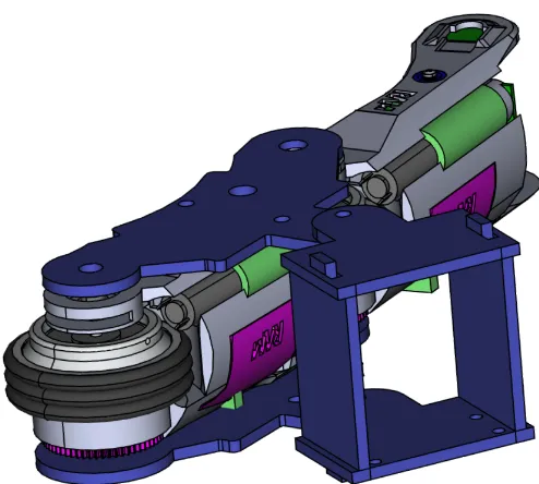
[image:28.612.170.417.428.650.2]

The 3D detection algorithm is tested with the rotating ‘LS02 Lidar’ sensor plus servo setup in 20 cm diameter pipe structures. This simply to test the ability of the algorithm to differentiate the types and correctly estimate their properties in a real life test environment. If satisfactory results can be obtained with the ‘LS02’ sensor, then it is tested on the PIRATE. As the setup with servo is too large to fit on the PIRATE it can only be fixed without the servo, meaning that only the 2D detection algorithm can be used. The ‘LS02 Solid State Lidar’ can be mounted on the PIRATE using the designed assembly depicted in figure 4.4. The mount can be rotated to the perfect orientation of the sensor, for the maximum detection of points on both sides of the pipe.

(29)

“Insanity: doing the same thing over and over again and expecting different results.”

— Albert Einstein

Results & Discussion

5.1 Simulation Results & Analysis

In this section the results obtained from simulations in Gazebo are presented and analyzed. The focus is on determining the limits, such as the accuracy and standard deviation, of both algorithms to calculate the pipe properties.

5.1.1 Analysis of the 2D Detection Algorithm Results

The 2D detection algorithm is tested by moving the sensor through several simulated pipe structures, while keeping its sensing plane horizontal. The results of these simulations are analysed next.

The first simulation is done to check the performance of the LS02 LiDAR in a 6 cm diameter pipe. It is already expected that little to no points can be detected due to the minimum range, considered 10 cm, of the sensor. The simulations show that, when placed exactly in the center of a straight pipe, the diameter can indeed be estimated accurately with about 12 points on each side of the pipe wall, as can be seen in figure 5.1a. If the pipe ends the distance to this end is also known, but the message to stop is only send when this distance is less than 30 cm. When the sensor moves to either side of the center, less points are detected on the side to which it moves and vice versa. A sharp bend cannot be detected as there are little to no outlying points1 for proper identification, as can be seen in figure 5.1b2. From this it can be presumed that junctions cannot be detected with the ‘LS02 Solid State 2D LIDAR’ in small diameter pipes, i.e. diameters less than its minimum range (10 cm).

(a) Graphical representation of the points detected in the straight section.

(b) Top view of the practical sensor near the bend.

Figure 5.1: Results of the 2D simulation tests in a 60 mm diameter pipe bend.

1_{Outlying points are those that are detected outside the known radius of the pipe.} 2

(30)

Master Thesis Results & Discussion

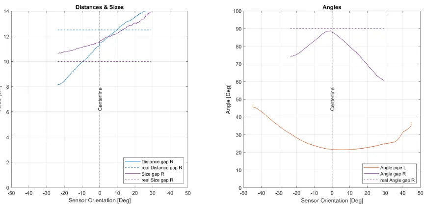
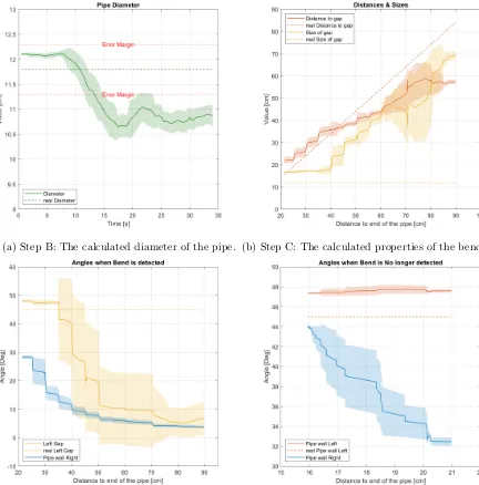
Therefore, the remaining 2D simulations are performed in pipes with 10 cm inner-diameter sections and using the ‘ideal LiDAR’ sensor specifications. The first test, to check the 2D detection algorithm, is done by moving the sensor towards a mitre bend on the right at a constant velocity. The test is done ten times to determine the accuracy and reliability of the algorithm. The results of these tests are combined and graphically presented in figure 5.2. The sub-figures present the working process of the algorithm, specifically showing the results of steps B and C as described in algorithm 1 (in section 3.2.2). The first graph, figure 5.2a, shows the diameter calculated at each position during step B. Here it can clearly be seen that the diameter is calculated accurately in a straight pipe section. Then, as the sensor moves closer to the bend, positioned at approximately 118 cm, the diameter decreases. The standard deviation, presented by the shaded area, of these calculations remains somewhat constant at around 0.4 mm, which is very acceptable. Once the diameter reaches the error margin, at about 30 cm before the bend, the algorithm goes to step C to start the gap detection. The resulting calculated properties are plotter in the graphs according to their units (in figure 5.2b). The plot on the left, Distances & Sizes, shows the calculated diameter of the bend (size gap R) and the distance to its entrance with respect to the overall position of the sensor. The plot on the right, Angles, shows the estimated absolute angles of the pipe and bend with respect to the pipe centerline at each sensor position. As one could have expected, the estimations are quite far from their actual values in the beginning, but significantly improve closer to the bend as more points of the bend are detected. In the Distances & Sizes plot, the error from the mean to the real value of the distance to the gap, drops from 3 cm at a position of 92 cm to nearly 0 cm at position 112 cm. For the size and angle estimations at the same positions, the error drops from 4 cm to nearly 0 cm and 12° to 0.05°, respectively. Both the distance and size calculations have a standard deviation of ±6 mm over the complete motion, whereas that of the angle of the gap decreases significantly from±4.5° to 0°. Furthermore, as no gap is detected on the left side, the algorithm outputs the estimated angle of the left pipe wall (Angle gap L). It is expected that, while driving towards a mitre bend on the right, the pipe wall on the left eventually forms an arc with a slope of about 45°. This is indeed observed in the graph. Note that, here the standard deviation actually increases closer to the bend. This due to the effect that small differences in the position of each detected point has on the slope estimation through linear regression.

Overall, it can be said that at a distance of≈14 cm before the structure3_{, the pipe}

prop-erties are calculated correctly with the preferred accuracy (as stated in section 3.1.2). The reliability of the algorithm is also satisfactory, with a maximum standard deviation of±6 mm for the distance and size and a maximum of±5° for the angles, over ten test runs4.

Next, the effect of sensor misalignment on the calculations and output of the 2D detection algorithm is analyzed. This is done in the same 10 cm inner-diameter pipe structure with a 90°bend to the right. When positioning the sensor block against either side of the pipe wall5 and driving towards the bend, the results are as expected. Further away from the bend, in the

x-direction, more points are detected inside the gap. Thus resulting in better estimations of the gap properties. Closer to the bend, on the other hand, little to no points can be detected because the pipe wall is in the way. This, of course, resulting in very bad estimations of

3_{This distance is at the 104 cm position in the graphs of figure 5.2.} 4

Note that these results are specif to the pipe diameter (10 cm) in which the tests are done.

(31)

(a) Step B: The calculated diameter of the pipe.

[image:31.612.191.394.167.371.2]

(b) Step C: The calculated properties of the detected structure.

Figure 5.2: Simulation results of the 2D detection algorithm (steps B & C) while moving the ‘ideal LiDAR’ through a 10 cm pipe towards a 90° bend to the right.

(32)

the pipe properties. The exact results of this test are appended in figure D.12 and further analysis on these is left for interpretation by the reader. Instead, the effect of misalignment is analyzed by fixing the y-position of the sensor block on the centerline, and moving it in thex-direction with constant velocity toward both sides of the pipe wall. From the previous test, in figure 5.2, they-position is chosen at 106 cm, this is at a distance of approximately 12.5 cm to the entrance of the bend. The moving average of each of the pipe properties, calculated during this test, is plotted in the graphs in figure 5.3. As expected, the error, of the calculated properties with the real values, decreases when moving further away from the bend in the x-direction. The real problem arises when the sensor is positioned close to the bend or junction that is to be detected. Therefore, the graphs to the right of the centerline are of more interest. The error of the distance and size seems to grow linearly, whereas that of the angle grows exponentially while moving closer to the bend. This can be attributed to the fact that the angle estimation highly depends on the number of points detected in the gap. From the graphs, it can be deduced that the maximum misalignment the sensor may have in the x-direction, to remain within the required accuracy, is ±2 cm. Meaning that, while facing forward, the sensor should not be positioned further than 2 cm away from the center of a 10 cm diameter pipe to properly detect gaps on either side, 12 cm before these are reached. If the gaps need to be detected earlier this misalignment should, of course, be less.

(33)

[image:33.612.90.521.136.345.2]

[image:33.612.89.521.456.667.2]

Figure 5.3: The calculated bend properties while translating the sensor block from left to right with respect to the pipe centerline. These results are obtained with the 2D detection algorithm in a simulated 10 cm inner-diameter pipe with a 90° bend to the right.

(34)

5.1.2 Analysis of the 3D Detection Algorithm Results

Next, the ability to detect and identify pipe structures in different directions is also tested and the results are analyzed. Therefore, the 3D detection algorithm is first put to test in a 10 cm inner-diameter straight pipe with a simple reduction, a type 1 pipe structure as specified in section 2.2.1. The 45 % reduction of the diameter occurs over a distance of 20 cm, resulting in a 5.5 cm straight pipe section after the reduction. A picture of the simulated environment is appended (see figure D.10). For this simulation the ideal LiDAR sensor is used and moved towards the reduction at increments of 5 cm after each full 180° rotation of the servo. During the simulation it is observed that the reduction is first detected just 5 cm before the reduction starts. This relatively late detection of the section is due to the fact that the average radius is calculated from all detected points at each measurement instance. Because the reduction is not abrupt, but occurs gradually over the 20 cm distance, the change in radius is also small. When a type 1 pipe section is detected, the algorithm returns the smallest diameter detected and the minimum distance to this. This is generally considered to be the new pipe diameter after the reduction and the distance to the end of the reduction. During the simulation the sensor block is moved towards the end of reducing part of the pipe. The results obtained during this motion are analyzed and tabulated in table 5.1. As the distance to the end changes while moving through the reduction, the mean and standard deviation of this are not included.

Table 5.1: Analysis of the pipe properties calculated by 3D detection algorithm at distances of 25 cm to 5 cm before the end of the reduction is reached.

Reduction

(Type 1) Mean

Standard Deviation

Average Error

from the real value Unit Estimated Distance to

the end of the reduction x x 1.88 cm

Estimated Diameter of the

pipe after the reduction 5.38 0.1 0.12 cm

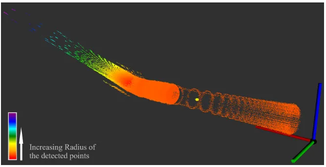
Due to the PIRATE its clamping method, it can easily adjust when driving through reductions. So detection of these does not have much added value for autonomous motion. The detection of bends, however, does provide notable information that will aid in autonomous navigation of these. Therefore, the 3D detection algorithm is tested in a simulated 45° pipe bend. The pipe is rotated in a way such that the direction of the bend, with respect to the horizontal initial position of the sensor (its virtualx-axis), is 136°. The point cloud obtained while driving through this pipe structure, seen in figure 5.5, gives a clear visualisation of this. The bend is first detected approximately 30 cm before its entrance. The algorithm correctly identifies the bend, as a type 2 pipe structure, up to approximately 15 cm before its entrance. The pipe properties that are estimated within this region are analyzed, of which the results are presented in table 5.2. Note that when a type 2 section is identified the diameter is assumed to remain the same, therefore it is disregarded in the analysis. A noteworthy observation from the analysis of the data, is the increasing error of the estimated direction while approaching the bend. The error increases6 from just 3° to 28°, resulting in the large statistical values

6

(35)

[image:35.612.135.469.215.386.2]

for the direction in table 5.2. This is, likely, due to the fact that the direction is estimated using the center of the estimated ellipse from the outline points. Since these points might not exactly form a circle or ellipse from every measurement, the resulting estimation varies every time. The statistical properties of the estimated angle of the bend, on the other hand, are satisfactory during the entire detection. It should also be noted that when the sensor is very close to the bend, this gets identified as a type 1 section. This is expected, since the algorithm cannot identify an outline anymore.

Figure 5.5: 3D Point cloud, with respect to the global (x,y,z) coordinate frame, obtained while driving through a simulated 45° pipe bend. The pipe is oriented with the bend at an angle of 44° from the positive y-axis.

Table 5.2: Analysis results of the pipe properties estimated by the 3D detection algorithm in the range between 30 cm and 15 cm before the entrance of the 45° bend.

Bend (Type 2)

Mean Value

Standard Deviation

Average Error

from real value Unit Distance to the

Entrance x x 4.04 cm

Direction 147.33 11.14 11.35 °

Angle 45.87 1.31 1.2 °

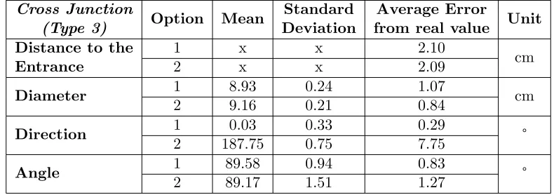
Lastly, the 3D detection algorithm is put to the ultimate test of identifying multiple junctions. For this test a horizontally oriented cross-junction, a type 3 pipe structure, is simulated in Gazebo. During this test, the structure is detected when the sensor is at a distance between 15 cm and 5 cm from the center of the cross-junction. The algorithm again correctly identifies the structure and returns that there are three possible options. The estimated properties of the first two options are analyzed, whereas the third option is simply the option to keep going forward. The results of the statistical analysis are presented in table 5.3. In these results it is noticeable that the standard deviations are much smaller than before. This because, the outline of pipe sections orthogonal to the centerline7 has a more elliptical form than that of pipe sections at a different angle from the centerline. Due to

(36)

[image:36.612.103.498.187.326.2]

this, the similar ellipse parameters are estimated at each position of the sensor (within the detection range).

Table 5.3: Statistical analysis results of the estimated pipe properties, calculated by the 3D detection algorithm at distances between 15 cm and 5 cm from the center of a cross-junction.

Cross Junction

(Type 3) Option Mean

Standard Deviation

Average Error

from real value Unit Distance to the

Entrance

1 x x 2.10

cm

2 x x 2.09

Diameter 1 8.93 0.24 1.07 cm

2 9.16 0.21 0.84

Direction 1 0.03 0.33 0.29 °

2 187.75 0.75 7.75

Angle 1 89.58 0.94 0.83 °

2 89.17 1.51 1.27

5.2 Practical Test Results & Analysis

As it shown in the simulations that the detection algorithms are able to detect and (to a certain extend) correctly identify the pipe structures, the next step is to test the algorithms in a practical environment using the ‘YDLidar’ for the 2D algorithm and the ‘LS02 Solid State 2D LIDAR’ for the 3D detection algorithm.

5.2.1 Results & Analysis of the 2D Detection Algorithm

(37)

region, the standard deviation and error of the angle of the bend are 2° and 3°, respectively. To show what happens when the sensor near the bend, the graph on the right in figure 5.6c is included. Even though the structure is no longer identified as a bend, the angle of the bend is still accurately estimated as ‘Pipe wall Left’.

(a) Step B: The calculated diameter of the pipe. (b) Step C: The calculated properties of the bend.

[image:37.612.84.516.180.618.2]

(c) Step C: The calculated angular properties of the detected structure.

Figure 5.6: Statistical analysis of the pipe properties estimated with the 2D detection algo-rithm (steps B & C) while moving the ‘YD LiDAR’ through a 12 cm diameter pipe towards a 45° bend to the left. The graphs present the moving mean and corresponding standard deviation (the shaded area) of the pipe properties.

(38)

returned properties and presented in the graphs in figure 5.7. These show a similar trend of the estimated data, to that of the previous experiment. As the pipe structure is symmetric, one could expect similar estimations for the left and right side properties. The trend of the data is indeed similar, but the values deviate as clearly seen in figure 5.7b. This can be attributed to the fact that exact alignment of the sensor along the centerline of the pipe is very difficult.

(a) Step B: The calculated diameter of the pipe. (b) Step C: The calculated angular properties of the junction.

[image:38.612.269.513.209.413.2]

(c) Step C: The calculated properties of the junction.

(39)

5.2.2 3D Detection Experiments

[image:39.612.196.409.453.667.2]

The 3D detection algorithm is put to the test, using the pragmatic setup described in sec-tion 4.3. Even though it takes quite some time for the servo motor to make a 180° rotation with 2° increments, the experiment is executed well. This execution again consists of incre-mentally moving the sensor setup towards the (90°) bend after each rotation. Because of the actual minimum distance of the ‘LS02’ sensor and the larger setup the test is performed in a 20 cm diameter pipe. During this test the poor performance of this sensor is clearly observed, unfortunately. Primary stationary tests of the sensor showed that it has a constant measure-ment error of 2 cm. This is taken into consideration in the 3D detection algorithm, but to no avail. Of the 6 different positions at which the algorithm is run to detect and identify the bend, the identification is correct twice. Specifically at distances of 90 cm and 50 cm from the bend, the algorithm returns the properties of a type 2 identified structure. These estimated properties, however, are questionable. Especially because, the angle of the bend is both times estimated to be almost parallel to the centerline. Whereas the direction estimation is is about 20° one time and 250° the next. At the other positions, at which the setup is placed inside the pipe, the algorithm identifies a type 1 structure. At a position at which the bend is still clearly visible, determined from inspection of the measured points visualized in RViz, the special points are collected. Recall that the special points are those that form the inliers, outliers and outline in the 3D detection algorithm (as mentioned in section 3.2.2. These are plotted in figure 5.8, which clearly shows the constant error of the sensor measurements from actual value. Furthermore, it can be seen that the maximum outliers are indeed detected inside the bend8. From the figure the cause of the misidentification can also be seen, i.e the wrong detection of the outline points on both sides of the pipe wall.

Figure 5.8: The ‘Special Points’ obtained with the 3D detection algorithm during a practical test in a 12 cm diameter with a bend.

(40)

5.3 Results Conclusion & Discussion

The many experiments, both in simulation and practice, show that the algorithms are indeed capable of detecting, identifying and estimating different pipe structures, using a 2D Light Detection and Ranging (LiDAR) scanner. The distance at which the structures are first detected and correctly identified, depends on the diameter of the pipe in which the sensor is placed and the actual structure to be detected. For small (<10 cm) diameter pipes, type 2 and closed ended type 3 structures can be identified at a distance of 20 cm from the pipe. In pipes with a slightly larger diameter this distance is already seen to increase to 40 cm. Reductions and open ended type 3 structures9, on the other hand, may be more difficult to detect. This because of the small change in the average diameter of the pipe and the late detection of outlying points with a significantly larger radius than the pipe wall. The threshold for a point to be an outlier can be lowered in the algorithms, to provide earlier detection of junctions. But this has to be done with caution as sensor measurement noise and misalignment may cause erroneous collections of points. The estimations of the properties generally improve closer to the structure, and the standard deviations tend to decrease. To increase the reliability and robustness of the algorithm a kind of trust factor can be included. This factor should place more weight on the accuracy of the estimated properties obtained closer to the structure. Then when the operator makes a choice for the PIRATE, the average over all calculations, each multiplied with its own weighting factor, can be determined. This average then provides the final information that can be used in the motion primitives for the PIRATE.

Regarding misalignment of the sensor, it is deduced that a maximum position error, with respect to the centerline, of 20 % of the inner-pipe diameter is allowed. For the sensor ori-entation, the allowable misalignment is ±4° from the forward facing orientation along the centerline. To avoid the calculation errors from large misalignment from the centerline, feed-back from the configuration of the front module and sensor in the pipe should be implemented. The algorithms already include the possibility to set the exact position with respect to which the LiDAR measurements are obtained. When placed on the PIRATE, the position and ori-entation of the sensor can easily be obtained from the encoders and the IMU. Feedback on the exact position of the sensor in the pipe is especially important for proper transformation of the points for 3D detection of structures. When the sensor is aligned within its allowable error margins, the 3D detection algorithm provides adequate results of the physical pipe properties. The estimations of sharp bends and junctions are returned with the least amount of error. When junctions and bends at smaller angles from the centerline are encountered, however, the algorithm fails to correctly estimate the direction and size. This due to the fact that the outlines of these sections are not exactly elliptical, resulting in different and wrong ellipse estimations at each measurement instant. To improve the estimation of the shape from the detected outlines, one can take the eccentricity of the estimated ellipse into account and the deviation of the fitted ellipse to the outline points.

Tests on the PIRATE itself were not executed due to the disappointing performance of the ‘LS02 Solid State Lidar’. Recall that the PIRATE can currently only operate in pipes of maximum 12 cm diameter. Tests with the ‘LS02’ sensor showed that little to no points can be detected on both sides of the pipe wall in these pipes. Therefore, the actual performance of the detection algorithms when integrated on the PIRATE remains to be confirmed.

(41)

“I did then what I knew how to do. Now that I know better, I do better.”

— Maya Angelou

Concluding

6.1 Conclusion

This project aimed at developing an on-board sensing system for the Pipe Inspection Robot for AuTonomous Exploration (PIRATE) to enable navigational autonomy, i.e. the ‘Decision Support’ level of autonomy, through complex pipe structures. The baseline for this devel-opment was set by the main research question and the aid of two sub-questions. To recall the first sub-question, “Is a 2D LiDAR sensor sufficient to recognize a mitre bend in a closed pipe structure?”,it can be concluded that a 2D LiDAR is indeed capable of detecting these, as wel as other more complex pipe structures. This conclusion is based on the simulated and practical test results obtained with the 2D detection algorithm. Which show that junctions and bends can already be identified correctly 40 cm before they are reached. This distance may vary depending on the exact structure and diameter of the pipe. The capability of the 2D LiDAR to detect bends and junctions does has its requirements and limits, however. Apart from the fact that the minimum range of the sensor should be less than the diameter of the pipe, it should also be well aligned with the centerline of the pipe. When no feedback from the configuration is available, the sensor must be aligned within a distance of 20 % of the diameter and a maximum 4° deviation from the centerline. The error of the results obtained from both algorithms when the sensor is well aligned, is tabulated in table 6.1. During the research, it was also found that quantitative methods can best be utilized to determine the type of structure and its properties. This, because LiDAR sensors provide quantitative data that only has to be transformed to a specific coordinate frame, after which interpretation of the data is straightforward. To specifically answer the second sub-question, “Which methods can be used in a detection algorithm for the PIRATE to navigate closed pipe structures, with readings from sensors available on the system?”, only measurement data obtained from the LiDAR has been implemented until now. The developed algorithms utilize the method of collecting the measured points into blobs of three different categories, i.e. inliers, outline or outliers. Then, based on the specific characteristics of each, the type of pipe structure is identified and its properties are calculated. The ability to include feedback from the IMU and angle sensors is included in the algorithms but has not specifically been tested. The parameters that are to be obtained from the data of these sensors, i.e. pipe diameter and orientation of the PIRATE, are currently set manually. Finally to answer the main research question,

How can the PIRATE efficiently detect and identify complex closed pipe structures, for autonomous navigation through these, using an on-board sensing system?

(42)

[image:42.612.170.436.148.260.2]

Master Thesis Conclude

Table 6.1: Accuracy of the calculated pipe properties with both detection algorithm in the optimal detection range, i.e. at distances between 40 cm and 10 cm before the structure.

Maximum error from the actual value 2D detection

algorithm

3D detection

algorithm Unit

Diameter 6 1 cm

Distance 5 4 cm

Angle 3 2 °

Direction x 11 °

Overall it is concluded that Light Detection and Ranging provides an efficient way to detect and identify landmarks in closed pipe structures. As long as a sensor with a small enough minimum range and wide Field of View is used for the pipe diameters in which the Pipe Inspection Robot for AuTonomous Exploration (PIRATE) should operate. The created detection algorithms are then able to properly determine the type of pipe section approached and its properties. The actual ‘Decision Support’ level of autonomy for the PIRATE has not been realized as yet.