Splitting of separatrices in area preserving maps close to 1:3 resonance

(1)

warwick.ac.uk/lib-publications

A Thesis Submitted for the Degree of PhD at the University of Warwick

Permanent WRAP URL:

http://wrap.warwick.ac.uk/88465

Copyright and reuse:

This thesis is made available online and is protected by original copyright.

Please scroll down to view the document itself.

Please refer to the repository record for this item for information to help you to cite it.

Our policy information is available from the repository home page.

(2)

M A

E

G

NS I

T A T

MOLEM

U N

IV

ER

SITAS WARWICEN

SIS

Splitting of separatrices in area-preserving maps

close to 1:3 resonance

by

Giannis Moutsinas

Thesis

Submitted to the University of Warwick for the degree of

Doctor of Philosophy

Mathematics Institute

(3)

(4)

Acknowledgments

First and foremost I wish to thank my supervisor Vassili Gelfreich for his patience,

support, guidance and illuminating explainations throughout the course of the last

4 years. Without him this thesis could have never been completed.

I would like to thank Arturo Vieiro for our many discussions and for helping me

understand some numerical aspects of the separatrix splitting but also arranging my

accomodation in my visit in Barcelona. I am also thankful to David Sauzin for his

explaination on resurgence. I have discussed parts of the work presented here with a

number of people and I would especially like to thank Ernest Fontich, Narc´ıs Miguel

Ba˜nos and Dayal Strub. I thank Anatoly Neishtadt and Adam Epstein for agreeing

to be my examiners. I also thank Magdalena Zajaczkowska for proofreading the

text.

(9)

(10)

Declarations

I, Giannis Moutsinas, declare that to the best of my knowledge this work is

orig-inal work obtained in collaboration with my supervisor, Vassili Gelfreich, unless

otherwise stated, cited, or commonly known

The material in this thesis has not to my knowledge been submitted for any other

degree either at this university (the University of Warwick) or any other university.

At the time of submission none of the work within this thesis has appeared or been

(11)

(12)

Abstract

We consider a real analytic family of area-preserving maps on C2, fµ, depending

analytically on the parameter, such that f0 is a map at 1:3 resonance. Such maps can be formally embedded in an one degree of freedom Hamiltonian system, called

the normal form of the map. We denote the third iterate of the map by Fµ=fµ3.

We show that given a certain non degeneracy condition on the mapF0, there exists a Stokes constant, θ, that when it does not vanish, it describes the splitting of the separatrices that the normal form predicts. We show that this constant can be

approximated numerically for any non-degenerate map F0.

For a non-vanishing and small enough µ, we show that if the Stokes constant does not vanish the separatrices split. Moreover, let Ω be the area of the parallelogram

defined by the 2 vectors tangent at the two separatrices at a homoclinic point. For

any M ∈Nwe have the estimate

Ω(µ) =

M

X

n=0

ϑn(logλµ)n+O (logλµ)M+1

!

e−

2π2

logλµ_.

In this equation λµ is the largest eigenvalue of the saddle points around the origin

(13)

(14)

Chapter 1

Introduction

One of the fundamental questions of Hamiltonian systems is the one about the

stability of periodic orbits. One way to answer this question is the first return map or Poincar´e map. This map is constructed as the intersection of a periodic orbit in

the state space of a Hamiltonian system with a certain lower-dimensional subspace

transversal to the flow of the system.

As an example, we consider a 2 degrees of freedom Hamiltonian system. The state

space of such a system is of dimension 4, but since we know that the Hamiltonian function is an integral of the system, by choosing a value for this function we can

look at the surface that this defines and this drops the dimension to 3. Then we

assume there exists a periodic orbit on this 3 dimensional surface. We choose a point of this periodic orbit and we consider a plane transversal to the orbit.

In order to construct the first return map we choose a point on the plane and we

let the flow evolve until its trajectory crosses the plane again. Then we define the

map such that the image of the point we chose under the map is the point of the first crossing. Notice that the intersection of the periodic trajectory and the plane

is a fixed point of the map and usually it is considered to be the origin of the plane.

This procedure is shown in Figure 1.1. This map, now defined on a neighbourhood of the origin on the plane, can be shown to preserve area, see [Arn90]. Formally we

have the following definition.

Definition 1.1. Let V ⊂_R2 _{open with 0} _∈_V _{and let}_f _:_V _→

R2 be a function

analytic in V, such that f(0) =0. If detf0(x) = 1 for all x∈V, then we say that

f is an area-preserving map of the plane.

(15)

[image:15.595.113.269.138.293.2]

Figure 1.1: The construction of the first return map.

fixed point we have the following cases:

• λ1, λ2 ∈R,λ16=λ2 calledhyperbolic fixed point,

• λ1,2 = e±i2πρ, ρ∈(0,1₂)\Q callednon-resonant elliptic fixed point,

• λ1,2 = e±i2πρ, ρ∈(0,1₂)∩Q calledresonant elliptic fixed point,

• λ1,2 =±1 calledparabolic fixed point.

In a neighbourhood of a hyperbolic fixed point the map is the time-1 flow of a

Hamiltonian system around a saddle. In a neighbourhood of a non-resonant elliptic

fixed point the map is approximately a rotation, in general with a non-constant angle. The other two cases have many subcases. We will consider the case where

λ1,2 = e±i2π/3. An elliptic point with these eigenvalues is called an elliptic point at 1 : 3 resonance.

At first glance, resonant elliptic points seem rather improbable since they have codimension 1. However in order to construct the map we fix the value of the

Hamiltonian. Naturally we can change this value and by the implicit function

theorem we get the existence of a periodic trajectory in nearby values. So the value of the Hamiltonian is a “natural” unfolding parameter of the map which implies

(16)

1.1 Non-integrability of Hamiltonian systems

The phenomenon we will study here is connected with the non-integrability of

Hamiltonian systems and was first observed by the French mathematician Henri Poincar´e around 1890 when investigating the stability of the solar system. Poincar´e

considered the system formed by three bodies: Sun, Earth and Moon, under the

action of Newton’s laws of gravity. In an attempt to prove the stability of the three body system, he used perturbation series and realized its divergent character due

to the presence of a transverse homoclinic orbit [Poi90]. He also noticed that a

small differences in the initial positions or velocities of one of the bodies would lead to a radically different state when compared to the unperturbed system, what is

now commonly known as deterministic chaos. Poincar´e realized that a small

per-turbation can destroy a homoclinic connection and its place is taken by a region where the stable and the unstable manifolds intersect in a highly non-trivial way.

He was even able to prove for a concrete example that the width of this region was

exponentially small with respect to the size of the perturbation.

This splitting of separatrices is exactly the phenomenon we are interested here. We will give some brief historical remarks and we encourage the reader to see the survey

by Gelfreich and Lazutkin [GL01] for a more detailed exposition of the theory until

2000.

Splitting of separatrices in area-preserving maps

The obvious way to address the above question of stability of periodic orbits in two degrees of freedom systems is to look directly at the map.

The first map to be treated was the Chirikov standard map, defined on the torus

by



 

x

y



 7→



 

x+y+εsin(x)

y+ε sin(x)



 .

For ε = 0 the standard map is integrable but for ε >0 the homoclinic separatrix splits. An asymptotic formula for the splitting in the standard map was published

by Lazutkin in 1984 in a pioneering article, see [Laz03] for the english translation. However the proof was incomplete and it was completed and published by

(17)

[HM93], using Ecalle’s theory of resurgent functions. However their work was purely formal without rigorous proof.

Neishtadt, [Nei84], proved that the splitting in the difference of the two separatrices

of analytic maps close to identity admits an exponentially small upper bound. Later

Fontich and Sim´o, [FS90], using Lazutkin’s methods gave a sharp upper bound.

Using the theory of resurgent functions, Gelfreich and Sauzin proved for an instance

of the H´enon map at 1:1 resonance that the splitting of separatrices is exponentially small and provided the first asymptotic term for it, see [GS01].

More recently Mart´ın, Sauzin and Seara have studied the splitting of separatrices in perturbations of the McMillan map, see [MSS11a] and [MSS11b]. Their approach

combined the theory of resurgent functions with Lazutkin’s original ideas.

A paper, [Gel02], was published by Gelfreich stating the first asymptotic term for the

resonances 1:1, 1:2 and 1:3. However the only proof on these results published until now is a preprint by Br¨annstr¨om and Gelfreich [BG08]. There the authors derive

and prove the asymptotic formula for area-preserving maps near a Hamiltonian

saddle-centre bifurcation.

Non-autonomous perturbation of flows

An other way to address the above question is to embed the first return map into the flow of an non-autonomous Hamiltonian system of one degree of freedom. This

enables the usage of methods developed for differential equations and more results

are available. This flow can be written as a periodic time dependent perturbation of an one degree of freedom Hamiltonian system. More precisely, we describe this

system with the help of the Hamiltonian function

H(µ, ε;x, y, t) =H0(x, y) +µ H1(x, y,_εt, ε, µ),

withH1(x, y, t, ε, µ) periodic int.

A natural question in this setting is whether homoclinic or heteroclinic connections

that exists in the unperturbed system persist in the perturbed one.

The case where onlyµis considered to be a small parameter was solved using the so called Melnikov method, see [Mel63]. In this case we can reparametrize time such thatε= 1. Then for the separatrices of the system it holds

(18)

We define the Melnikov function by

M(t0) :=

Z ∞

−∞

{H0, H1}|W0(t−t0),tdt,

where {H, G} is the Poisson bracket of H and G. For the difference between the two separatrices at t0, measured in a coordinate system that usesH0 as the first of its coordinates, we get that the difference in the first component is

d(t0) =µ M(t0) +O(µ2).

However, when bothµandεare considered small, thenεcannot be ignored. These systems are called rapidly forced systems since the period of the perturbation

be-comes arbitrarily small.

Nekhoroshev, [Nek77], showed that in many degrees of freedom Hamiltonian sys-tems, the phase space can be covered by domains where the system behaves as if it

was integrable for some time. He showed that this time is exponentially large with

the size of the perturbation. Neishtadt showed in [Nei84] that d actually admits an upper bound that is exponentially small withε. Neishtadt’s results were refined by Treshchev in [Tre97]. Fontich based on Lazutkin’s ideas, [Fon95], showed that

the exponent depends on the location of the singularities in the parameter of the unperturbed separatrix.

In rapidly forced systems the Melnikov function can become exponentially small with ε, but since the error term is polynomially small in µ, the error can become bigger than the approximation. This situation can be avoided of course when µ

is a function of ε which decreases exponentially as ε goes to 0. Then the error is also exponentially small and the Melnikov method can still be applied. It was

shown by Gelfreich in [Gel97b] that this can be relaxed to a polynomial dependence,

|µ|6Cεp_{, with}_p _{big enough.}

Stronger results have been proved in specific systems. Poincar´e [Poi93] discovered the phenomenon of splitting by looking at the system described by the Hamiltonian

y2

2 + cosx+asinxcos

t ε.

He proved that in this system the splitting is exponentially small and he derived the

(19)

Treshchev [Tre96] and Gelfreich [Gel97a] independently showed that by obtaining a different asymptotic formula using the averaging method with a continuous

pa-rameter.

The most studied system has been the rapidly perturbed pendulum with a

pertur-bation only depending on time,

¨

x= sinx+µεηsint

ε.

Many authors have published on this, gradually strengthening the result, see [HMS88],

[Sch89], [DS92], [Ang93], [EKS93], [Gel94] and [Swa96].

Recently Gaiv˜ao and Gelfreich [GG11] used the generalized Swift-Hohenberg

equa-tion as an example to show the transversality of the homoclinic soluequa-tions near a Hamiltonian-Hopf bifurcation.

Baldoma, Fontich, Guardia and Seara [BFGS12] showed that in systems where

H0 = y

2

2 +V(x) with V an algebraic or trigonometric polynomial and |µ| 6Cε

η_,

the Melnikov method can be applied ifη >0. Moreover, they also showed that the Melnikov method fails whenp becomes zero and they derived the first term of the asymptotic series in this case.

Splitting of separatrices in physics

The same phenomenon has been studied in physics although in a different

frame-work. The common technique there is truncating an asymptotic series in the optimal order and then showing that the remainder is exponentially small. This technique

is called asymptotics beyond all order or superasymptotics, see [Ber91], [STL12] or

[IL05].

There exist many examples of problems for which asymptotic power series methods lead to divergent series. Oppenheimer [Opp28] while investigating a phenomenon

in quantum physics known as the Stark effect, demonstrated that the lifetime of a

certain quantum state was inversely proportional to a quantity exponentially small with the strength of the electric field applied at the system.

Kruskal and Segur [KS91] demonstrated that the geometric model for dendritic crystal growth fails to produce needle crystal solutions due to exponentially small

effects, a byproduct of the breakage of a heteroclinic connection. This work has

(20)

to certain singularly perturbed systems. Examples of application of this method include surface tension and wave formation [GJ95], [YA97], [Tov00], [VdBK09]),

crystal growth [CM05] and optics [CK09]. More information about applications of

exponentially small splitting to mechanics, fluids and optics can be found in the survey of Champneys [Cha98].

In his book [Lom00], Lombardi puts the superasymptotics into rigorous arguments

that can be used to solve many problems in exponentially small phenomena. He

did that by reducing the problem to the study of certain oscillatory integrals which describe the exponentially small terms.

1.2 Measuring the splitting of separatrices

Until now we talked about the splitting of separatrices without defining concretely what it means. The reason for this is that there are a handful of different quantities

that were used to measure it. Let us describe them.

• The splitting angle. Measuring the angle that the two separatrices create at

their intersection is an intuitive idea, since it cannot vanish when they meet

transversally. However there are a few disadvantages: computing the angle requires the definition of a Riemannian metric, it depends on the homoclinic

point chosen, and finally a symplectic change of variables changes also the

angle.

• Thesplitting amplitude is defined as max_t∈{t0,t0+1}|W

+

ε (t)−Wε−(t)|, wheret0 corresponds to a homoclinic point, W_ε+(t0) =Wε−(t0). However the splitting amplitude has the same disadvantages as the splitting angle.

• The homoclinic invariant, Ω, was introduced by Lazutkin in [GLS94]. It is

defined by Ω = ω( ˙W_ε+(t0),W˙ε−(t0)) and it represents the area of the par-allelogram formed by the tangent vectors to the separatrices at a point of intersection. The homoclinic invariant has the same value on all homoclinic

points and it is invariant under canonical changes of coordinates.

• The area of a crescent. We choose a homoclinic point ph and we look at

the segments of the separatrices bounded byph and its image under the map

Fε(ph). If the separatrices split, there are finitely many points of

intersec-tion between these two segments. We choose two neighbouring ones and we

measure the area the two separatrices define. This area is invariant not only

(21)

• The width of the instability region. One can show using KAM theorem, that

the closure of the separatrices is contained in a domain bounded by invariant

curves, each of which is diffeomorphic to a circle. One can speak of the

‘last’ invariant curve bounding the so-called instability region. The splitting of separatrices can be characterized by the width or the area of this region.

Note that the width is not an invariant.

The last quantity is harder to estimate than the preceding ones. The relationship

between the splitting amplitude and the width of the instability region was estab-lished by Lazutkin [Laz90] for the standard map, and a generalization of this result

was obtained by Treshchev [Tre98].

In the present analysis we will use Lazutkin’s homoclinic invariant to measure the

splitting.

1.3 Normal form of maps close to 1:3 resonance

An interesting class of area-preserving maps is the maps tangent to identity. The

definition is given below.

Definition 1.2. Let f be an area-preserving map of the plane, if f(0) = 0 and

f0(0) is the identity then we call f a tangent to identity map.

For any tangent to identity area-preserving map, there exists an one degree of

freedom Hamiltonian system, such that the map can be formally embedded in

its flow. This implies that such map can always be approximated with arbitrary precision by a flow.

LetV be a neighbourhood of the origin inC2 andI a neighbourhood of the origin in R. Letfµ:V →R2 be a real-analytic, area-preserving map for all µ∈ I. Moreover

let fµ(0) = 0, f00(0) have eigenvalues e± = e±2πi/3 and fµis C∞ inµ.

Theorem 1.3 (Birkhoff normal form). There is a formal canonical change of

co-ordinates Φsuch that the mapN = Φ◦f0◦Φ−1 commutes with the rotation R2π/3,

i.e: N ◦R₂_π/₃ =R₂_π/₃◦N.

The mapN is called theBirkhoff normal form off0 and the mapR−2π/3◦N is tan-gent to identity. Since a tantan-gent to identity map can be formally represented as the

(22)

H such that

N =R₂_π/₃◦φ1_H,

where φ1_H is the time-one flow of H. The corresponding vector field is usually called Takens normal form vector field, see [Tak74]. The Hamiltonian inherits the

symmetry of the normal form:

H◦R2π/3=H.

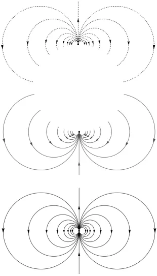
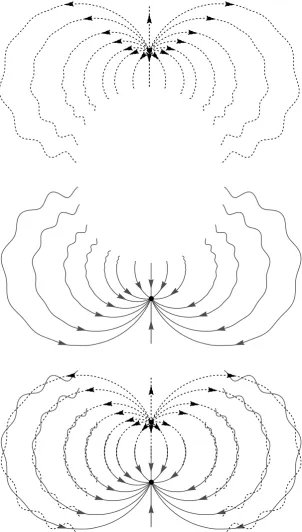
So H is a formal integral ofN and by changing back to the original coordinates we get a formal integral of f0. Note that if the map f0 is not integrable,H cannot be convergent. In the middle figure of Figure 1.2 the level lines of the third order of this Hamiltonian are shown.

The formal Hamiltonian H is not defined uniquely so there is room for further normalization.

Proposition 1.4([GG09]). Letf0 be as above. Then there is a formal Hamiltonian

H and formal canonical change of variables which conjugates f0 with R2π/3 ◦φ1H.

Moreover, H has the following form:

H(x, y) = (x2+y2)3A(x2+y2) + (2x3−6xy2)B(x2+y2), (1.1)

where A and B are series in one variable with real coefficients:

A(I) = X

k>0

k6=2 mod 3

akIk, B(I) =

b0 6 +

X

k>1

k6=2 mod 3

bkIk

and the coefficient of A and B are uniquely defined if b0 6= 0.

For the coefficient b0 it holds b0 = 6|h30|, where h30 is the 3rd order coefficient in Birkhoff normal form Hamiltonian.

For a map, fµ, close to the resonance it holds:

Proposition 1.5 ([GG09]). Let fµbe as above and let the coefficientb0 for the map

f0 not vanish. Then there is a formal Hamiltonian H and formal canonical change

of variables which conjugates fµ with R2π/3◦φ1H. Moreover, H has the following

form:

(23)

Figure 1.2: The normal form of the unfolded 1:3 resonant map.

where A and B are series in two variables with real coefficients:

A(µ, I) = X

k,m>0

k6=1 mod 3

ak,mIkµm, B(µ, I) =

b0,0 6 +

X

k,m>1

k6=2 mod 3

bk,mIkµm,

with b0,0 = b0 and a0,0 = a1,0 = 0. Moreover the coefficients of these series are

unique.

1.4 Splitting of separatrices

The normal form predicts that close to resonance there are heteroclinic connections

between the three saddle points. However since the convergence of the normal form is not given, it is natural to ask whether this prediction is correct. In his classical

book Mathematical Methods of Classical Mechanics, V.I. Arnol’d conjectures that

this is actually not true.

Since the class of maps is bigger than the class of flows, he states that there is no

reason to expect all maps to act like flows. One of the implications of this is that the heteroclinic connections are not actually present. He also argues that the difference

between the two separatrices has to be exponentially small since the normal form

cannot detect it at any order and of course the presence of splitting implies that the normal form is divergent.

We will see that the splitting of the separatrices close to the 1:3 resonance is

dom-inated by the splitting at exactly 1:3 resonance and that there is a transversal

intersection in generic maps close to 1:3 resonance.

In order to simplify our analysis, we defineFµ:=fµ3, i.e. the third iterate of the map

(24)

[image:24.595.137.518.98.224.2]

Figure 1.3: The separatrices of the normal form.

with the rotation by 2π/3, the normal form Hamiltonian for Fµ is just the normal

form Hamiltonian for fµ multiplied by 3.

In Figure 1.3, the fixed points with the separatrices are shown. Notice that the separatrices of the flow are not invariant sets forfµ, sincefµmaps one to the other,

but are invariant sets forFµ. From now on we will consider the mapFµ.

We see that at the resonance the stable and the instable separatrices of the origin do

not meet at all so of course they do not split. To see the splitting at the resonance

we need to study the map in a complex neighbourhood of the origin. This is done trivially since the map is considered to be analytic around the origin.

Map at resonance

We consider the vertical set of separatrices at resonance. Both of them are curves of

dimension 1 inR2, so when we complexify the map they become curves of complex

dimension 1 in C2. So we can draw the dynamics close to a separatrix by taking

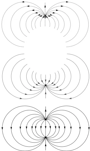
the projection on one of the coordinates. In Figure 1.4 we see what happens in the

case of an integrable map. In this case the normal form is convergent and the map is just the time-1 flow of a Hamiltonian. This means that the invariant lines of the

unstable and the stable separatrices coincide and all but the points on the real line

have the fixed point as alpha and omega limit set.

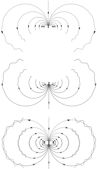
On the other hand, when we consider a non-integrable map, we see that close to

the real separatrix the dynamics is similar to the integrable case but as we move away the invariant lines start to oscillate. We see in Figure 1.5 that when the two

separatrices are drawn together the splitting is apparent. It should be noted here that the splitting of the separatrices does not happen only on the plane that they

(25)

[image:25.595.112.423.110.654.2]

(26)

[image:26.595.169.481.109.651.2]

(27)

plane of projection.

Map close to resonance

As we saw, for a map close to resonance two saddle points appear on the vertical set of separatrices. The separatrices are again curves of dimension 1 inR2 and curves

of complex dimension 1 in C2 when the complexified map is considered. As in the

resonant case we can draw the invariant lines on the projection of the separatrix on

the second coordinate. In Figure 1.6 the integrable case is shown. We see that again

the stable and unstable invariant lines coincide and every point but a half-line have the unstable fixed point as alpha limit set. Similarly, every point but a half-line

have the stable fixed point as omega limit set.

In the non-integrable case an oscillation appears in both separatrices away from the

fixed points, see Figure 1.7. Comparing the Figures 1.5 and 1.7 we see that even

though at a neighbourhood of the resonant fixed point the change is dramatic, away from it the dynamics do not change a lot.

The separatrices are analytic functions so of course their difference is also an analytic function. With analytic functions being global objects, it is reasonable to expect

that the difference close to the fixed points can be calculated by the difference away from them. Then since the dynamics away from the fixed points do not change

significantly with the unfolding, it is reasonable to expect that the difference at the

resonance dominates the difference of the unfolding. We will show that is actually the case.

1.5 Results

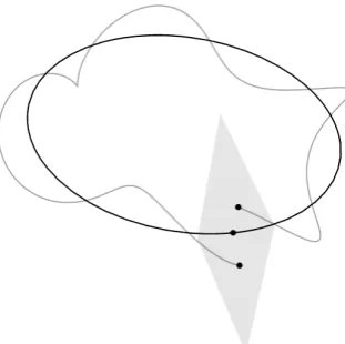
Once a non-integrable map gets unfolded the splitting of the separatrices appear on R2. As shown in Figure 1.8 the heteroclinic connections get destroyed and

separatrices meet transversally in a complicated way. In order to measure this

splitting we will use the homoclinic invariant1 Ω.

In this section we summarize the results of this thesis. In Chapter 3 we deal with the

map at resonance. In Chapter 4 we derive the asymptotic formula for the homoclinic

1_{One could argue that the word that should be used here is heteroclinic instead of homoclinic.}

There are basically two reasons for this choice. One is historical, since this is the name originally used. The second is that this connection could actually be viewed as a homoclinic one. Recall that the hyperbolic points are fixed points of the mapFµand not of the mapfµ. For the mapfµthese

(28)

[image:28.595.168.480.116.641.2]

(29)

[image:29.595.117.420.112.645.2]

(30)

[image:30.595.192.461.115.382.2]

Figure 1.8: The splitting of the triangle that separatrices form.

invariant. Finally in Chapter 5 we provide a numerical method to compute the Stokes constant of a resonant map.

The theorems of the following chapters are repeated here however the wording has been slightly changed to avoid referring to notions that have not been defined yet.

The reader should treat this section just as a summary of the results and is advised to refer to the respective chapters for any other purpose.

Assumptions on the map

Let V be a neighbourhood of the origin inC2 and I a neighbourhood of the origin

in R. Let fµ :V → R2 be a real-analytic, area-preserving map for allµ ∈ I. Let

moreoverfµ(0) = 0,f00(0) have eigenvaluese±= e±2πi/3 and fµbe analytic around

0 inµ. We assume that the coefficientb0,0 of the normal form does not vanish. We defineFµ=fµ3. From now onFµwill denote the third iterate of an area-preserving

(31)

Chapter 3 results

Let F0 agrees at least up to order 4 with the normal form of Proposition 1.4. We consider the equation

W(t+ 1) =F0(W(t)). (1.2)

Theorem 3.1. There exists a unique formal solution with real coefficients,

W(t) =



 

0

− 1

b0t 



+O(|t|

−3₎_∈ 1

tC[[

1

t]]

2_,

of equation (1.2) and any other formal solution of the form W0(t) = (0,− 1

b0t) +

O(|t|−2₎ _{can be written as} _W₍_t₊_c₎ _{for some}_c_∈

C. Moreover there exists a formal solution with real coefficients, Ξ˜ ∈t2C[[1_t]]2, of the equation

X(t+ 1) =F₀0(W(t))·X(t),

such that

˜ Ξ(t) =



 

b0t2−18b_b12 0

+ 24b21

b5 0

t−2

−8a0

b3 0 t

−1





+O(|t|

−3₎_,

and det(˜Ξ(t),W˙(t)) = 1.

The Borel transform ofW is a function,Wˆ, analytic around the origin with singu-larities at2πiZ∗ and is of exponential type along any path that crosses the imaginary

axis finitely many time and does not go to infinity vertically.

The Borel-Laplace summation of W gives two solutions of the equation (1.2), W+

and W−, that satisfy limt→±∞W±(t) = 0. There exist two complex constants, θ

and ρ, such that for any t∈ {z∈C:|Re (z)|61,Im (z)<0}, with |t| big enough, it holds

W+(t)−W−(t)e−2πit

θΞ(˜ t) +ρW˙(t)

+O(t7e−4πit)

and

θ= lim

t→+∞e

2πt_ω₍_W+₍₋_i_t₎₋_W−₍₋_i_t₎_,_W_˙ −₍₋_i_t₎₎_.

(32)

Chapter 4 results

Notice that for the next theorem we assume the map is as described above but also

we have an extra assumption that the Stokes constant of the resonant map does

not vanish.

Theorem 4.2. Let Fµ be an area-preserving map that agrees with the normal form

stated in section 1.3 up to degree 4 and that F0 is the third iterate of non-degenerate

area-preserving map at resonance 1:3. For µ 6= 0, let λµ denote the largest

eigen-value of its saddle points and letΩbe the Lazutkin homoclinic invariant of the map.

If the Stokes constantθof the resonant map does not vanish, then there existµ0>0

and real constants ϑn such that for anyµ∈(−µ0, µ0)\{0} and any M ∈N it holds

Ω(µ) =

M

X

n=0

ϑn(logλµ)n+O (logλµ)M+1

!

e−

2π2

logλµ_.

Moreover ϑ0 = 4π|θ|.

Chapter 5 results

Let WN denote the truncation of the formal seriesW to orderN.

Theorem 5.3. ForM, N ∈_N,M, N >2, there existst0>1such that forwN(t) =

WN(t) +O(|t|−N−1),wM(t) =WM(t) +O(|t|−M−1)and allt∈ {C:|t|> t0,Re (t)6 0}, the following are true.

1. The limit W−(t) := limm→∞F0m(wN(t−m)) exists, is an analytic function

and

lim

m→∞F

m

0 (wM(t−m)) = lim

n→∞F

n

0(wN(t−n)).

2. W−(t) =F0(W−(t−1)).

3. There existsC1 >0 such thatkW−(t)−wN(t)k∞6C1|t|−N−1.

4. There existsC2 >0 such that for all m∈N

kW−(t)−F₀m(wN(t−m))k∞6C2|t−m|−N+1.

5. There existsC3 >0 such that for all m∈N

(33)

We use this theorem to assess the expected error of numerical experiments and we show numerically that for an instance of the H´enon map,

H:



 

x

y





7→R2π/3· 

 

x

y−x2



 ,

(34)

Chapter 2

Preliminaries

In this chapter the main ideas behind resurgence will be presented. Most of the

results stated here will not be proved, the reader is referred to the bibliography for the proofs. The theory originated from the work of ´Ecalle [ ´Eca81]. Unfortunately

his books are not available in English. An introduction in English can be found

in [Sau08, Sau13a, SS96]. In this exposition we will loosely follow [Sau08] and [Sau13a]. In [SS96] the definition of resurgent functions is aimed to be used in

ODEs and PDEs and it is slightly more restrictive but also slightly stronger. A

proof of existence of symmetric paths can be found in [Sau13b]. The content of sections 2.5.7 and 2.5.8 is original work unless it is specified otherwise.

2.1 Notation

We denote by N the set of all positive integers, the same set with 0 added will

be denoted by N0. By R an C we denote the sets of real and complex numbers

respectively. By R+ we denote the set of all positive reals andR+0 is the set of all

non negative reals. Similarly we define R− and R−0. We denote by Dr(z) the open

disk centered at z of radius r and by D∗r(z) the same disk minus its center. We

denote by ω the standard symplectic form on C2.

Throughout this text we will use the pair of variablestandsas duals of each other. The Laplace transform will always be applied to a function of s and the Borel transform will always be applied to a function or a formal series of 1_t. Moreover

when we talk about the ring of formal or convergent series it will be implicitly

(35)

We will abuse the notation sn. This will have both the normal meaning of the number that s represents raised to the power of n, but also it will represent the function s7→ sn. Finallyf(x)2 will denote the product f(x)·f(x) and f2(x) will denote f◦f(x). This notation extends to any integer.

2.2 Useful functional spaces

2.2.1 The space Cω₍

C) of entire functions

Let Cω(C) be the space of entire functions equipped with the topology generated

by the family of seminorms

kfk

Dn := sup

s∈_Dn

|f(s)|,

withn∈N. Under this topology Cω(C) becomes a Fr´echet space.

2.2.2 The spaces Bn(Dr)

Letr >0 andg(s) be a function analytic onDr. We definekgkn:= sups∈Dr|s

−n_g₍_s₎_|_,

n∈_N. This implies |g(s)|₆|s|n_k_g_k

n. We defineBn(Dr) :={g∈Cω(Dr) :kgkn <

∞}.

It is trivial to check that k·k_n is a norm on Bn(Dr). Let {gn}n>0 be Cauchy in

B_n(Dr),

|gn(s)−gm(s)|6|s|nkgn−gmkn6r n_k_g

n−gmkn.

So Cauchy inBn(Dr) implies uniform Cauchy in Dr, which implies that the limit is

inB_n(Dr), thus (Bn(Dr),k·kn) is Banach.

Evidently iff ∈ Bn(Dr) then around the origin f is of the formc sn+O(sn+1). So

iff ∈ B_n₊_m(Dr), then kfkn6rmkfkn+m. This implies that for n, m > 0 it holds Bn+m(Dr)⊂ Bn(Dr).

Notice that the space B_n(Dr)× Bn(Dr) ≡ Bn(Dr)2 with the norm k·k×2,n defined

by

k(f, g)k_×₂_,n := max{kfk_n,kgk_n}.

(36)

θ

Figure 2.1: The Laplace transform of a function of exponential typeτ in the direc-tion θ gives rise to a function analytic in the half-plane{Re (teiθ)> τ}.

2.3 Classical Borel and Laplace transforms

In this section we present some elementary properties of the Laplace transform and

of its formal inverse, the Borel transform. For an in depth treatment the reader should refer to one of the numerous books on the subject, we mention [Sch99] as

an example. The Laplace transform is usually defined as an integral from 0 to ∞.

Here we will use a slightly more general definition.

Definition 2.1. Let θ ∈ R and ˆφ be such that r 7→ φˆ(reiθ) is analytic on a

neighbourhood of R+ and |φˆ(s)|6Ceτ|s|. Functions with this property are called functions of exponential type along the direction θ. If the previous bound holds in every direction, we just say that the function is of exponential type. Moreover if τ0

is the infimum of all such τ we say that the function is of exponential typeτ0. We define the Laplace transform in the direction θas the linear operator Lθ,

Lθ_φ_ˆ₍_t_{) :=}

Z eiθ∞

0

e−tsφˆ(s)ds.

The function Lθ_φˆ_{is analytic on the half-plane Re (}_t_eiθ₎_{> τ}0_{, see Figure 2.1.}

We define the convolution of two functions by

f∗g(s) =

Z s

0

(37)

θ

1

θ₂

Figure 2.2: If ˆφis analytic and of exponential type τ in a sector, then the domain of analyticity of L(θ1,θ2)_φˆ_{is the union of all possible half-planes.}

The Laplace transform transforms convolution to multiplication. i.e.

Lθ_{[ ˆ}_f_∗_f_ˆ_{] =}_Lθ_{[ ˆ}_f_]_·_Lθ_{[ ˆ}_f_]_.

If the function ˆφis analytic in a sector{s∈_C|θ1 <args < θ2}, with θ2−θ1 < π, and is of exponential typeτ in that sector, then the Laplace transform converges on anyθin the sector and the functionLθ1_φˆ_{is the analytic continuation of}Lθ2_φˆ_{. So}

we can define the functionL(θ1,θ2)_φˆ_{which is analytic in the union of the domains}

of analyticity of Lθφˆfor all θ in the sector, see Figure 2.2. We can define L(θ1,θ2)_φˆ_{also when} _{π < θ}

2−θ1 <2π. The situation is essentially the same with the only difference that the functionL(θ1,θ2)_φˆ_{might be multivalued.}

Let θ ∈ (0,π₂). If ˆφ is of exponential type τ in the sectors Sθ = {s ∈ C| −θ <

args < θ} and S−θ ={s ∈ C|π−θ < args < π+θ} but it is not of exponential

type in C\(Sθ)∩S−θ, then one can define L(−θ,θ)φˆ and L(π−θ,π+θ)φˆ. See Figure

2.3. However at the points t where both are defined their difference cannot be identically equal to 0.

If ˆφhas a pole at finite distance from the origin, then its Taylor series has a positive but finite radius of convergence. This implies that the Laplace transform of its

Taylor series, applied termwise, has 0 radius of convergence.

Let C[[s]] denote the space of formal power series of s with complex coefficients.

We denote byt−1

(38)

[image:38.595.229.424.97.298.2]

Figure 2.3: The domains ofL(−θ,θ)φˆand L(π−θ,π+θ)φˆ.

constant term.

Because R₀∞s_nn_!e−tsds=t−n−1 for Ret >0, we have for any θ

Lθ

sn n!

(t) =t−n−1, Re (teiθ)>0.

Using this we define the formal Laplace transform Lθ :C[[s]]→t−1C[[t−1]].

Definition 2.2. The formal Borel transform is the linear operator

B: φe(t) = X

n>0

cn

tn+1 ∈t

−1

C[[t−1]] 7→ φˆ(s) = X

n>0

cn

sn

n! ∈C[[s]].

Notice that the Borel transform is formally the inverse of the Laplace transform. This means that since the Laplace transform turns convolution into multiplication,

the Borel transform turns multiplication into convolution.

If φe has a positive radius of convergence, if for example it converges for t−1 < ρ,

then ˆφdefines an entire function of exponential type ρ−1.

Let φe∈t−1C[[t−1]] be divergent and let ˆφ=Bφe∈C[[s]] have a positive radius of

convergence. Still it may happen that ˆφextends analytically and is of exponential type in sectors. In these cases the Laplace transform converges in each sector but

generally each sector defines a different function. This implies that we can possibly

(39)

We denote by E the analytic continuation of a function defined as a convergent power series around the origin. We define

I(θ1,θ2)₌L(θ1,θ2)_{◦ E ◦}B

to be the Borel Laplace summation over the sector (θ1, θ2). Similarly if for some ˜

φ ∈t−1C[[t−1]], I(θ1,θ2)[ ˜φ] is a function analytic at a domain like the one in right

figure of 2.2, we say that ˜φis Borel-Laplace summable.

The Borel Laplace summation is regular, i.e. it sends a convergent series to its

function. It is linear and it commutes with multiplication, differentiation, integra-tion, translation of the argument and composition. These imply that if ˜φ satisfies formally some analytic equation then its Borel Laplace sum satisfies the same

equa-tion.

2.4 Formal series

2.4.1 The multiplicative ring _C[[t−1]]

Recall that byC[[t−1]] we denote the space of complex formal power series of t−1.

Addition, multiplication by a constant and multiplication of two series can be

de-fined in a straightforward way. Let ˜A(t) = P

n>0ant

−n _{and ˜}_B₍_t_{) =} P

n>0bnt

−n_,

c∈_C. Then

cA˜(t) =X

n>0

c ant−n,

˜

A(t) + ˜B(t) =X

n>0

(an+bn)t−n,

˜

A(t) ˜B(t) =X

n>0

n

X

m=0

ambn−m

!

t−n.

Division ˜A(t)/B˜(t) is well defined if and only if b0 6= 0. These imply that C[[t−1]]

is a ring. Moreover the usual derivation dt := _dd_t acts on C[[t−1]], so C[[t−1]] is a

differential ring.

We define the valuation onC[[t−1]] as the map val :C[[t−1]]→N∪ {∞} by

(40)

and val(0) :=∞. With this we can define a metric on C[[t−1]] by

µ( ˜A,B˜) := 2−val( ˜A−B˜).

Using this metric we can define a topology under which C[[t−1]] is complete. In

particular in this topology if a map from C[[t−1]] to C[[t−1]] is such that any given

coefficient of the result depends on finitely many coefficients of the input then the

map is continuous.

Example 2.3. We will see that multiplication inC[[t−1]] is a continuous operation.

Let ˜AN(t) =PNn=0ant−n. Then we have

˜

AN(t) ˜B(t) =

X

n>0

n

X

m=0

am·bn−m·1{0,...,N}(m)

!

t−n,

where1{0,...,N}is the indicator function of the integers from 0 toN. We see that for

anyn6N then-th coefficient of the product ˜AN·B˜agrees with then-th coefficient

of ˜A·B˜. This implies that

µ( ˜A·B,˜ A˜N ·B˜)62−N−1,

so

lim

N→∞

˜

AN(t) ˜B(t) = ˜A(t) ˜B(t).

2.4.2 The convolutive ring _C[[s]]

We defined t−1C[[t−1]] as the space of formal series without constant term, which

is a maximal ideal in C[[t−1]]. The formal Borel transform maps t−1C[[t−1]] into C[[s]].

The spaceC[[s]] has a similar structure asC[[t−1]] but instead of considering it as a

ring with multiplication, we consider it as a ring with convolution. More precisely we define

C[[s]] = (

X

n>0

an

sn n!

an∈C, ∀n∈N )

and by the usual definition of convolution we get

sn n! ∗

sm m! =

sn+m+1

(41)

So for ˆA,Bˆ ∈C[[s]] we get

ˆ

A∗Bˆ(s) =X

n>0

n

X

m=0

ambn−m

!

sn+1

(n+ 1)!.

Since the formal Borel transform satisfiesB[ ˜A·B˜](s) =B[ ˜A]∗B[ ˜B](s), it respects the ring structure ofC[[t−1]]. However it is not a ring homomorphism sinceB[1](s)

is not defined. Moreover, even if we restrict our view onC[[s]] it is not obvious how

to define a convolutive unit there. So we considerC[[s]] as a ring without identity.

Operations on C[[t−1]] can be pulled back intoC[[s]]. We get the following lemma.

Lemma 2.4. Let A˜ ∈ _C[[t−1]]. Assuming that both sides are well defined and

defining Tc[ ˜A](t) = ˜A(t+c), we get

• B[dtA˜](s) =−sB[ ˜A](s),

• B[d−_t1A˜](s) =−1

sB[ ˜A](s),

• B[TcA˜](s) = e−csB[ ˜A](s) for all c∈C,

• B[tA˜](s) = dsB[ ˜A](s).

Remark. Using the above lemma one could write

B[1](s) =B[t·1_t](s) = dsB[1_t](s) = ds1 = 0.

This hints that a convolutive unit cannot be defined using this definition of Borel

transform.

The spaceC[[s]] happens to be too big for our needs, so we consider a smaller one,

namely C{s}, the space of convergent series around the origin. We have that

ˆ

A(s) =X

n>0

an

sn

n! ∈C{s}

if and only if there exist M, α > 0 such that for alln∈_N,an6M αnn!. The fact

thatB−1[ ˆA](t) =P

n>0ant−n−1 motivates the following definition.

Definition 2.5. LetC[[t−1]]1denote the space of all formal power seriesPn>0ant−n

for which there existM, α >0 such that an6M αnn! for alln∈N. This space will

(42)

2.5 Resurgence

We will introduce the idea of resurgent functions as a way to define B[1](s). This is not to imply that this was the historical reason, however it helps by placing the theory into context.

In order to define B[1](s) we need to extend the classical definition of the Laplace transform and to this end we define first the space of singularities.

2.5.1 The space of singularities

In order to define the space of singularities we need some technical definitions.

First we need the definition of the Riemann surface of the logarithm and then the definition of a spiraling neighbourhood of the origin.

The Riemann surface of the logarithm

By the Riemann surface of the logarithm, let it be denoted by ˜C, we mean the

universal cover of C∗ = C\{0} with base point at 1. In other words, we consider

the set P of all pathsγ : [0,1]→C∗ with γ(0) = 1 with the equivalence relation ∼

of homotopy with fixed endpoints, namely

γ0 ∼γ1 ⇐⇒ ∃H : [0,1]×[0,1]→C∗ continuous, with H(0,·) =γ0, H(1,·) =γ1,

H(σ,0) =γ0(0), H(σ,1) =γ0(1)∀σ∈[0,1].

Since the endpointγ(1) depends only on the equivalence class and not on the chosen representative, we can define the projection

π : ˜C→C∗, γ 7→γ(1).

To define a Riemann surface structure on ˜C we need first to define a Hausdorff

topology. This is done by taking a basis {_D˜r(γ)|γ0 ∈ C˜,|π(γ)−π(γ0)| < r} with

˜

Dr(γ) the set of the equivalence classes on ˜C classes of all paths γ0 obtained as

concatenation of a representative of γ and a line segment starting from π(γ) con-tained in Dr(π(γ)), the open disk of radius r centered at π(γ). Then each basis

element, π, induces a homeomorphism πγ,r : ˜Dr(γ) → Dr(π(γ)) and that for two

basis element with nonempty intersection the mapπγ0_,r0◦π_γ,r−1 is the identity on the

(43)

manifold structure on ˜C.

Note that the fact that the base point is at 1 plays no special role in the construction of the surface and can be moved to any other point ofC∗.

An alternative way to construct this surface is through the exponential function, by defining ˜C:= exp(C) such that exp−1 : ˜C→C is a bijection. This method has

the advantage that we do not need to choose an arbitrary point in ˜C to act as a

base. However the construction through homotopies of path gives more insight into notions that will follow.

Spiraling neighbourhoods of the origin

A spiraling neighbourhood of the origin is in essence what we get if on the Riemann surface of the logarithm we restrict the distance we can move away from the origin.

Let h :R→ (0,∞) be continuous, then we define P as the set of all paths of the

form γ : [0,1]→ _C∗ _with _γ₍_s_{) =}_r₍_θs_)eiθs_{, for some}_θ _∈

R and r continuous, such

that 0< r(σ)< h(σ), σ ∈ _Rand r(0) = h(0)/2. As above, we consider the set of all homotopy classes of Pand we call it a spiraling neighbourhood,Vh. As above, V(h) can be given a local 1-dimensional complex manifold structure.

Similarly to ˜C, there is an alternative definition of V(h) through the exponential

function. For this we fixH:R→Rand we define

CH :={z∈C: Re (z)< H(Im (z))}

and

V(h) := exp(CH)

with h = exp◦H. As noted above, we will use the definition by homotopy classes of paths since it gives more insight in the present analysis.

The space of singularities

We denote by ANA the space of functions analytic in a spiraling neighbourhood of

the origin. Formally we have the following definition.

Definition 2.6. We consider the space of all pairs ( ˇf , h), with h : R → (0,∞)

continuous and ˇf :V(h)→_Canalytic, equipped with the equivalence relation

(44)

Then we define the space ANA as the quotient set.

We see by the above definition that functions which are analytic in a neighbourhood

of the origin are contained in the space ANA. To get the space of singularities we

need to mod out all regular functions from ANA.

Definition 2.7. We define the space SING = ANA/C{s} and we denote the

quo-tient map by

sing₀: ANA→SING, fˇ7→sing₀( ˇf) = ˚f .

Any representative ˇf of ˚f is called amajor of ˚f.

Example 2.8. We have sing₀(_es1₋₁) = sing₀(1_s) and sing₀(_ess₋₁) = 0.

Definition 2.9. The linear map defined by1

var : SING→ANA, f˚7→fˇ(s)−fˇ(se−2πi)

is called variation and ˆf = var( ˚f) is called the minor of ˚f.

Example 2.10. Let φ∈_C{s}. Then var

sing₀ φ(s) log(s)

= 2πiφ(s).

The kernel of var is the space of all power series ins−1convergent around the origin.

The algebra of singularities

The space SING can be turned into a convolutive algebra with a properly defined

convolution.

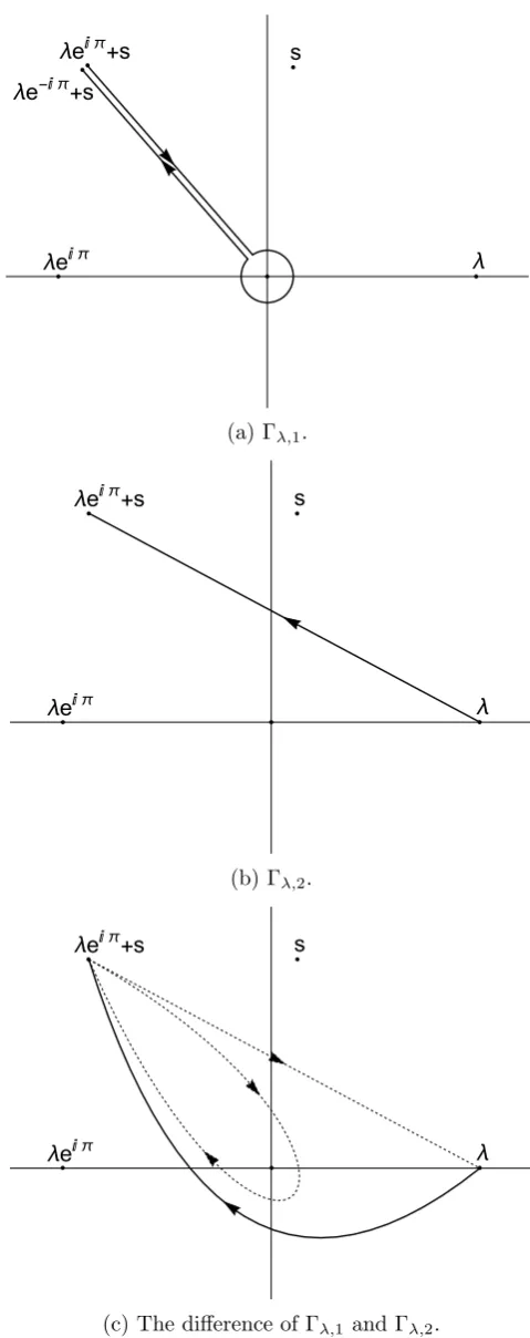
Definition 2.11. Let ˚f1,f˚2∈SING, with ( ˇf1, h1),( ˇf2, h2)∈ANA. Then chooseλ such that λ, λeπi∈ V(min{h1, h2}) and let

Hλ={s∈ V(min{h1, h2})|argλ <args <argλ+π}.

Then for s∈Hλ with|s|small enough we define

˚

f1∗f˚2(s) = sing0

Z

Γλ,1

ˇ

f1(σ) ˇf2(s−σ)dσ

!

,

1

There is an obvious abusion of notation here. Since e−2πi= 1, it is expected thatse−2πi=s. However instead of this obvious choice one should think ofse−2πi_{as the concatenation of 2 paths.}

(45)

s

λ λeⅈ π

λeⅈ π+s

λe-ⅈ π+s

(a) Γλ,1.

s

λ λeⅈ π

λeⅈ π+s

(b) Γλ,2.

s

λ λeⅈ π

λeⅈ π₊s

[image:45.595.146.386.96.701.2]

(c) The difference of Γλ,1 and Γλ,2.

(46)

with Γλ,1 as shown in Figure 2.4, and we call that the convolution of ˚f1 and ˚f2. Similarly, we can define

˚

f1∗ 2

˚

f2(s) = sing0

Z

Γλ,2

ˇ

f1(σ) ˇf2(s−σ)dσ

!

,

with Γλ,2 as shown in Figure 2.4. We will see that these two definitions coincide in

SING.

Notice that in Figure 2.4 where Γλ,1 is shown, the pointsλeπi+sandλe−πi+sare drawn as two distinct points for clarity even though they have the same projection.

Similarly the line segments to these points are drawn as distinct.

It is not hard to see that the two definitions of convolution coincide. Let’s consider

their difference ˚f1∗f˚2(s)−f˚1∗ 2

˚

f2(s). We see that this difference is an integral over a line that has both 0 and sat the same side. This means thatscan be pushed to 0 without problems which implies that the difference is analytic around the origin,

hence the two definitions coincide in SING. Similarly the definition of convolution does not depend on λ.

The convolution defined on SING is linear and symmetric. Moreover, we can easily guess a unit for this algebra by the Riemann integral, i.e. δ(s) = sing₀(₂_π1_i_s). Using the first definition of convolution we get δ∗f˚(s) = ˚f(s).

Multiplication of resurgent functions

Naturally we would like to extend the ring of resurgent functions to allow

multipli-cation. However we will see that the product of two resurgent functions cannot be defined uniquely.

Let ˚f and ˚gbe singularities and letφandψbe functions analytic around the origin. We could define

˚

f ·˚g= sing₀ fˇ·ˇg.

The problem that arises is that ˇf+φis also a major of ˚f so equally we have

˚

f·˚g= sing₀ ( ˇf+φ)·(ˇg+ψ)

= sing₀ fˇ·gˇ+ψ·fˇ+φ·ˇg+φ·ψ

= sing₀ fˇ·gˇ+ψ·fˇ+φ·ˇg

(47)

This shows that the product defined this way depends on the majors.

We can define the product of a singularity and an analytic function in a unique way,

φ·f˚= sing₀ φ·fˇ

.

However it holds that

s( ˚f∗˚g) = (sf˚)∗˚g+ ˚f∗(s˚g),

which means that the multiplication by s is a derivation for this algebra. This means that the multiplication by an analytic function should be thought as the

application of a differential operator of infinite order.

Correspondingly multiplication by 1_s acts as an integration. For a singularity ˚f we define

1

sf˚= sing0

1

s( ˇf+φ)

= sing₀1_sfˇ+φ(0)δ.

Since φis arbitrary,φ(0)δ has the role of the integration constant.

We can define uniquely the multiplication of 1_s with simple singularities by defining

P(1_s)·[φ= sing₀

1 2πiP(

1

s)·φ·log

and

P(1_s)·sing₀

Q(1_s)

= sing₀

P(1_s)·Q(1_s)

withP andQ a polynomials.

2.5.2 The generalized Borel and Laplace transforms

Let ˚f ∈ SING and take a major (or a representative of the class) ˇf ∈ ANA. We will assume that for some θ ∈ [0,2π] ˇf can be continued analytically along a neighbourhood of the half-line eθiR+ on two neighbouring sheets and its variation

is of exponential type along this line. Then we define

Lθf˚(t) =

Z

Γθ

(48)

where the path Γθ coming from infinity on the half-line eθiR+, circulating around

the origin and then going to infinity along eθiR. In Figure 2.5 this path is shown

with the two half lines separated for clarity.

θ

Figure 2.5: The path Γθused in the definition of the generalized Laplace transform.

Clearly the generalized Laplace transform does not depend on the major that is

chosen, so this is actually a definition for the Laplace transform of elements of

SING. We just need to check that this definition is compatible with the classical one.

Let ˆφbe a function analytic around the origin and of exponential growth along the half-line eθiR+. We define

b[ ˆφ](s) = ˆφ(s)log(s) 2πi and

[_φ_ˆ_{= sing}

0(b[ ˆφ]).

This can be considered as an embedding of C{s} into SING, because it satisfies

[_{( ˆ}_φ_∗_ψ_ˆ_{) =}[_φ_ˆ_∗[_ψ_ˆ_{. Then the classical Laplace transform,}_Lθ_{[ ˆ}_φ_](_t_{) =}R∞eiθ

0 e

−st_φ_ˆ₍_s_)d_s_,

and the generalized Laplace transform, Lθ_[[_φˆ_{], coincide. This implies the map}[ _is

the canonical embedding ofC{s}into SING and allows us to abuse the notation of

the 2 different Laplace transforms. We define

ANAreg=b(C{s}) and SINGreg=[C{s}= ANAreg/C{s}.

The formal Borel transform is defined analogously to the classical case as

B[t−n−1](s) =

[_sn

n! = sing0

sn n!

log(s) 2πi

.

Now for any θ ∈ _R we have Lθ_[ 1

2πis](t) =

R

Γθe

−st 1

2πisds = 1, so we can define

ˇ

(49)

and B[tn](s) =δ(n)(s) = sing₀ δˇ(n)(s) for any n∈N.

2.5.3 The Borel transform of Gevrey-1 formal series.

With the above generalization of the Borel transform we can map any element of

C[[t−1]]1 to ANA.

For ˜Φ∈_C[[t−1]]1 with ˜Φ(t) =c+ ˜φ(t), ˜φ∈ t−1C[[t−1]]1 we define

B[ ˜Φ](s) =cδˇ(s) + ˆφ(s)log(s)

2πi = ˇΦ(s),

with ˆφ(s)∈_C{s}given by the classical Borel transform. By taking the quotient we can map ˜Φ to SING, so we define

B[ ˜Φ] =c δ+[φˆ= ˚Φ.

Due to the properties of the Borel transform we see that it is a ring isomorphism

from C[[t−1]]1 toB[C[[t−1]]1]. We define

C[t][[t−1]]1=

(

P(t) + ˜Φ(t)

˜

Φ∈_C[[t−1]]1, ∃n∈N, P(t) =

n

X

k=1

pktk

)

and

ANAsim=

(

P[ˇδ] + ˆφ

∃n∈N, P[δ] =

n

X

k=1

pkδˇ(k), ∃φ˜∈C[[t−1]]1,B[ ˜φ] = ˆφ

)

.

The space ofsimple singularities is defined by the quotient

SINGsim= ANAsim/C{s}.

Then the following are true:

b:C{s} →ANAreg ⊂ANAsim,

sing₀: ANAsim →SINGsim,

var : SINGsim →_C{s}

and the map

(50)

is the identity map.

This happens because an element of ANAsimcan have 3 “components”: a convergent power series ofs, a polynomial ofs−1 _{and a logarithmic branching. The map sing}

0, which is the quotient map, kills the convergent power series. Then the variation kills

the polynomial and gives the difference of 2 consecutive branches of the logarithm, which is a regular function.

Remark. The statement of Lemma 2.4 holds in the general case. This can be seen

by considering the non-formal inverse Laplace transform. So in particular, it holds

when we consider the space C[t][[t−1]]1. For example we have

B[t−n] =B[t·t−n−1] = sing₀

ds

sn n!

log(s) 2πi

= sing₀

sn−1

2πin!+

sn−1

(n−1)! log(s)

2πi

= sing₀

sn−1

(n−1)! log(s)

2πi

.

Also

B[1] =B[t·t−1] = sing₀

ds

log(s) 2πi

= sing₀

1 2πis

=δ.

Remark. When we consider an ˚f in SINGsim we need not to define the value of

some ˇf on the base point of its spiraling neighbourhood, V(h_fˇ). This is because the variation of ˇf, i.e. the difference of two consecutive branches of ˇf, is always the same regular function no matter where we are on V(h_fˇ).

2.5.4 The Riemann surfaces R1 and R0

In this section we define two Riemann surfaces that are instrumental to the analysis.

The first one, R1, is the universal cover ofC\2πiZ. Formally we have the following

definition.

Definition 2.12. LetR₁be the set of all homotopy classes of continuously

differen-tiable pathsγ : [0,1]→_C\2πiZwithγ(0) = 1 and|γ˙|=|γ|. Letπ :R1→C\2πiZ,

γ 7→γ(1) be the projection map. We considerR1 as a Riemann surface by pulling back throughπ the complex structure ofC\2πiZ.

As in the Riemann surface of the logarithm, the base point 1 is not special and can be moved to any other point ofC\2πiZ. We define the principal sheet ofR1, denoted byRp₁, as the set of all homotopy classes of pathsγ : [0,1]→_C\(R−0 ∪ ±2πi[1,∞)),

(51)

The second surface, R0, is essentially R1 plus the origin. This means that we consider all paths that have a base point at 0 instead of 1. Formally we have the

following definition.

Definition 2.13. Let R₀ be the set of all homotopy classes of continuous and

piecewise continuously differentiable paths γ: [0,1]→Cwithγ(0) = 0, γ (0,1]⊂ C\2πiZand|γ˙|=|γ|plus the path0: [0,1]→0. Letπ:R0 →C\2πiZ∗,γ 7→γ(1)

be the projection map. We consider R₀ as a Riemann surface by pulling back

through π the complex structure ofC\2πiZ∗.

Notice that the preimage of the origin is just one point ofR₀, namelyπ−1(0) ={0}. Because of this the base point 0 is special forR0 and cannot be moved. Informally

R0 can be viewed as R1 with the origin attached. Similarly to R1 we define the

principal sheet ofR₀, denoted byRp₀, to be the set of all homotopy classes of paths

γ : [0,1]→_C\(±2πi[1,∞)), γ(0) = 0.

We can now consider the space Cω(R0). This is the space of functions analytic on

R0, which implies that they are also analytic around the origin. Similarly the space

Cω(R1) is defined to be the space of functions analytic onR1.

2.5.5 Resurgent functions

Resurgent functions should be thought of as singularities that can be extended

analytically along paths that avoid some points on C, where other singularities

appear. It is interesting to note that for any ˚f ∈ SING only the variation ˆf

plays a role when the singularity needs to be continued beyond its initial domain of

definition. This happens since any regular part around 0 that may have singularities elsewhere is killed by the quotient and the part that depends ons−1 can only have a singularity at 0. So only the variation can create singularities away from the origin.

In general the set of singular points is not defined a priori. However for the present

analysis, we do not need the theory in its full generality so we will predefine this set

of singularities. Usual choices for applications are 2πiZ,NandZ. Here the first

op-tion will be used. This means that from now on, every time that resurgent funcop-tions

are considered, it is implicitly assumed that they are functions with singularities at 2πiZ. This leads us to the following definition.

Definition 2.14. The space of resurgent functions RES is defined as the quotient

d

(52)

We have the inclusion map sing₀ :RESd →SING and we define res : SING→ RESd

as the inverse of sing₀ on its image. With this we can pull back convolution and

variation from SING inRES. The variation is trivially generalized ind RES, howeverd

there is an obvious problem with convolution. In SING convolution is well defined only close to 0. So it needs to be extended in a consistent way. This is done by

constructing symmetric paths, see Section 2.5.7. Using symmetric paths we get

that if Ω is a discrete subset of C that is invariant under addition then the space

of resurgent functions that have singularities on Ω are invariant under convolution,

see [Sau13b]. Obviously this is the case with 2πiZ.

Definition 2.15. We define the space ofregular resurgent functions as

d

RESreg = res◦sing₀◦b(Cω(R0))⊂RESd.

In simple words this definition means that we take an element of Cω(R0) and

multiply it by log(₂_πis) which makes it an element of Cω(R1). Then by applying sing₀ we get the quotient with C{s}. This is a singularity that can be extended

analytically toR₁so by definition is in sing₀(RES). Then the map res is well defined,d

so finally we get an element of RES. Evidently the map var :d RESd

reg

→_Cω₍_R

0) is the inverse of res◦sing₀◦band we see that RESd

reg

is isomorphic to Cω(R0). This

motivates the following definition.

Definition 2.16. We define the space ofregular resurgent power series as

g

RESreg=B−1hRESd

regi

⊂ 1

tC[[

1

t]]1.

To extend the algebraic structure of SING to RESd

reg

we use its isomorphism with

Cω(R0). On Cω(R0) we can use the classical definition of convolution close to the origin and we can extend it using symmetric paths. See next section. This implies

that we can pull back the operation of convolution onRESd

reg

and that this space is also stable under it. So both spaces are algebras with their respective convolutions

but without unit. Then the space RESg

reg

is stable under multiplication and of

course this makes it also an algebra without unit.

We can extend these spaces to turn them into algebras with units.

Definition 2.17. We define the space ofsimple resurgent functions as

d

RESsim=C1_s⊕RESd

reg

,

Splitting of separatrices in area preserving maps close to 1:3 resonance

warwick.ac.uk/lib-publications

A Thesis Submitted for the Degree of PhD at the University of Warwick

Permanent WRAP URL:

http://wrap.warwick.ac.uk/88465

Copyright and reuse:

This thesis is made available online and is protected by original copyright.

Please scroll down to view the document itself.

Please refer to the repository record for this item for information to help you to cite it.

Our policy information is available from the repository home page.

Splitting of separatrices in area-preserving maps

close to 1:3 resonance

Giannis Moutsinas

Mathematics Institute

Contents

Acknowledgments

Declarations

Abstract

Chapter 1

Introduction

1.1

Non-integrability of Hamiltonian systems

1.2

Measuring the splitting of separatrices

1.3

Normal form of maps close to 1:3 resonance

1.4

Splitting of separatrices

1.5

Results

Chapter 2

Preliminaries

2.1

Notation

2.2

Useful functional spaces

2.3

Classical Borel and Laplace transforms

2.4

Formal series

2.5

Resurgence