1
Faculty of Electrical Engineering,
Mathematics & Computer Science
Explaining system behaviour
in radar systems
Jan Thiemen Postema Master Thesis
August 2019
c
Thales Nederland B.V. and/or its suppliers.
This information carrier contains proprietary information which shall not be used, reproduced or disclosed to third parties without prior written authorization by Thales Nederland B.V. and/or its suppliers, as applicable.
Supervisors:
Summary
Radar systems are large, complex, and technologically advanced machines that have a very long life-span. This inherently means that there are a lot of parts and subsystems that can break. Thales Nederland develops a whole range of radar sys-tems, including theSMART-L MM, one of the world’s most advances radar systems,
capable of detecting targets at a distance of up to 2.000 kilometers. In order to aid the maintenance and repair of the radar it is equipped with a wide range of sensors, which results in a total of 1.100 sensor signals. The sensor signal are currently pro-cessed by two programs, a Built-In Test system, which gives alarms based on a set of rules and an outlier detection algorithm.
In the case of the anomaly detection algorithm the main shortcoming is the lack of explanations. Even though an outlier might be detected, there is still no explanation or label assigned to it. In order to resolve this shortcoming Thales wants to create a system which is capable of recognizing and grouping previously seen behaviour. This results in the following research questions:
1. To what extent can the system state be diagnosed automatically?
(a) Which techniques are available to diagnose the outliers and which are most suitable given the case described in Section 1.1 and the available data?
(b) How to assess the quality of the methods used to provide a diagnosis? (c) How do the methods selected in RQ 1.a stack up against each other
based on the metric found in RQ 1.b and training and diagnostic speed?
Based on an extensive literature review this report proposes to use a clustering algo-rithm to provide the explanations based on annotations. To find out which algoalgo-rithm works best, a total of seven combinations are tested. To find out if semi-supervised learning provides a substantial benefit over unsupervised learning for the case of Thales, this report also proposes a novel, semi-supervised constraint-based variant of the Self-Organizing Map (SOM) called the Constraint-Based Semi-Supervised Self-Organizing Map (CB-SSSOM).
CLASSIFICATION: OPEN III
The methodology with which these algorithms are tested consists of four steps, (1) pre-processing, (2) dimensionality reduction, (3) clustering and (4) evaluation. This is done on three synthetic data sets and one real data set. The latter is annotated manually by a domain expert to ease the evaluation.
A quick overview of the most important results can be found in Table 1. Most al-gorithms were tried both with and without dimensionality reduction performed by a Deep Belief Network (DBN).
The conclusion of the report is that unsupervised clustering is most likely not a vi-able option, although there is still some hope in the form of subspace clustering. However semi-supervised clustering did offer some promising results and could be a viable solution, especially when combined with Active Learning.
Algorithm Dimensionality Reduction u/i/s1 F-score
k-Means - u 0.2460
k-Means DBN u 0.4114
c-Means - u 0.2460
c-Means DBN u 0.2460
SOM - u 0.4020
SOM DBN u 0.2483
CB-SSSOM - i 0.5286
Table 1: Summary of the results obtained on a real data set
Contents
Summary ii
Glossary vii
1 Introduction 1
1.1 Motivation . . . 1
1.1.1 Annotations . . . 3
1.1.2 Explanations . . . 3
1.2 Data . . . 4
1.2.1 Challenges . . . 5
1.3 Research questions . . . 6
1.4 Research Method . . . 7
1.5 Report organization . . . 7
2 Background 8 2.1 Clustering methods . . . 8
2.1.1 K-Means . . . 8
2.1.2 Fuzzy c-Means clustering . . . 9
2.1.3 Self-Organising Maps . . . 9
2.1.4 Mixture Models . . . 10
2.1.5 Support Vector Machines . . . 10
2.1.6 Subspace clustering . . . 11
2.1.7 Semi-supervised clustering . . . 11
2.2 Dimensionality Reduction . . . 12
2.2.1 Principal Component Analysis . . . 12
2.2.2 Stacked Auto-Encoder . . . 12
2.2.3 Deep Belief Network . . . 13
3 Literature review 14 3.1 Fault diagnosis . . . 14
3.1.1 Spacecraft . . . 16
CONTENTS CLASSIFICATION: OPEN V
3.1.2 Power systems . . . 17
3.1.3 Bearings . . . 17
3.1.4 General datasets . . . 18
3.2 Performance metrics . . . 19
3.2.1 Supervised metrics . . . 21
3.3 Techniques . . . 22
3.3.1 Fault Diagnosis . . . 22
3.3.2 Classification in high-dimensional sparse data . . . 25
3.4 Summary . . . 27
4 Methodology 29 4.1 Data . . . 29
4.2 (1) Pre-processing . . . 30
4.3 (2) Dimensionality reduction . . . 30
4.4 (3) Clustering . . . 31
4.4.1 k-Means Clustering . . . 31
4.4.2 Fuzzy Clustering . . . 32
4.4.3 Self-Organizing Maps . . . 32
4.4.4 Constraint-Based Semi-Supervised Self-Organizing Map . . . 32
4.5 (4) Evaluation . . . 33
4.6 Hyper-parameter estimation . . . 34
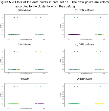
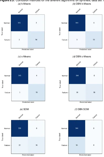
5 Results 35 5.1 Synthetic data set . . . 35
5.2 Real data set . . . 42
5.3 Runtime . . . 48
6 Discussion 50 6.1 Implications . . . 50
6.2 Issues . . . 51
7 Conclusion 54
References 57
Appendices
A Fault Diagnosis 106
VI CLASSIFICATION: OPEN CONTENTS
C Data 132
C.1 Synthetic data . . . 132 C.2 Real data . . . 135
D Constraint-Based Semi-Supervised Self-Organizing Map 138 D.1 Pseudo code . . . 139 D.2 Assumptions . . . 140
Glossary
AE Auto Encoder
AL Active Learning
ANN Artificial Neural Networks
ANWGG Adaptive Non-parametric Weighted-feature GathGeva
AP Affinity Propagation
BIT Built-In Test
BMU Best Matching Unit
CE Classification Entropy
C-L Cannot-Link
CB-SSSOM Constraint-Based Semi-Supervised Self-Organizing Map
CNN Convolutional Neural Network
D-S Dempster-Shafer
DAE Deep Auto Encoder
DBN Deep Belief Network
DT Decision Tree
EA Evolutionary Algorithm
EM Expectation Maximization
FDD Fault Detection and Diagnosis
FFNN Feed Forward Neural Network
VIII CLASSIFICATION: OPEN GLOSSARY
GA Genetic Algorithm
GG Gath-Geva
GK GustafsonKessel
HMM Hidden Markov Model
HUMS Health and Usage Monitoring System
k-NN k-Nearest Neighbour
LDA Linear Discriminant Analysis
LSTM Long Short Term Memory
M-L Must-Link
MLPNN Multi-Layer Perceptron Neural Network
MM Mixture Model
MRW Markov Random Walk
NMI Normalized Mutual Information
NN Neural Network
NWFE Non-parametric Weighted Feature Extraction
OAA One-Against-All
OAO One-Against-One
PC Partition Coefficient
PCA Principal Component Analysis
PSO Particle Swarm Optimization
PUFK Pearson VII Universal Function Kernel
RBF Radial Basis Function
RBM Restricted Bolzman Machine
GLOSSARY CLASSIFICATION: OPEN IX
RNN Recurrent Neural Network
SAE Stacked Auto Encoders
SC Subspace Clustering
SDAE Stacked Denoising Auto Encoder
SOM Self-Organizing Map
SVD Singular Value Decomposition
SVM Support Vector Machine
TL Transfer Learning
Chapter 1
Introduction
This document describes the results of my master thesis at the University of Twente, which forms the conclusion of the Master Computer Science with a specialization in Data Science. The master thesis is performed at Thales Nederland in Hengelo. Thales Group S.A. is a multinational company with over 80.000 employees that builds and develops electronic systems for many markets, including aerospace, fence, security and transportation. A large portion of the group’s sales are in de-fence, which makes it the tenth largest defence contractor in the world.
One of the subsidiaries that develops defence systems is Thales Nederland. This company that has its origins in the Hollandse Signaalapparaten B.V. primarily con-cerns itself with the development of combat management, radar and sensor sys-tems.
One of those radar systems is theSMART-L MM. This is one of the largest and most
advanced radar systems developed by Thales Nederland and can detect targets at a distance of up to 2.000 kilometers. This project will focus on theSMART-L MM.
1.1 Motivation
The SMART-L MM radar systems are complex and expensive machines that are
crucial to the operations of the defence forces. Therefore unexpected downtime will create serious issues for the operators. This is where the Health and Usage Moni-toring System (HUMS) team comes in.
HUMS is responsible for monitoring the complete radar system and giving alarms when a certain part is not functioning as expected. In order to do this a modern radar system has a large number of sensors that monitor many properties including the temperature of the cooling water and the electric current required by the mo-tor that rotates the radar. In the case of the SMART-L MM this results in a total of
about 1.100 sensor signals. Those signals are currently monitored by two separate
2 CLASSIFICATION: OPEN CHAPTER1. INTRODUCTION
computer programs. The first one is the traditional Built-In Test (BIT) program. This program is based around a predefined set of rules which it uses to fire alarms. So, if a certain sensor reading crosses a threshold value an alarm is fired. The BIT program also tries to find the origin of the problem and, if there are multiple alarms, to group them and find the possible causes. This is partly done based on rules and partly on a model of the radar system. These rules are entered through an elaborate set of Excel sheets and are then parsed into a set of if-else clauses.
The second program that monitors the sensor readings is an outlier detection sys-tem. This outlier detection is currently a univariate program that works based on a statistical model of the data. When the likelihood of seeing a certain value falls below a chosen threshold value an alert is send to the user through a monitoring dashboard. This program is slated to be extended by a multivariate outlier detection algorithm that should be capable of better handling the different usage states the radar is in, which have a large influence on its behavior. It should also be able to find correlations between different sensor readings. In the future Thales also wants to include the temporal aspects of the data in the detection algorithm.
The goal of this research is to explain system behaviour in radar systems, however this requires some further specification. A radar system, in this case, is a com-plete radar system such as the SMART-L MM, including all of its sub components,
1.1. MOTIVATION CLASSIFICATION: OPEN 3
1.1.1 Annotations
The HUMS team has also been developing an annotation server. This annotation tool is integrated in the monitoring dashboard and can be used by the operators to provide truth values by adding a label to a certain point in time or to an anomaly, or by giving feedback on an existing label, such as the BIT alarms. The user could for example say that an anomaly was indeed a failure. The operator of the radar could also say that the failure was not legitimate and give it a label. There are four types of annotations, which are defined below.
• General; An annotation that spans a certain time period but is not assigned to
a specific element or time series
• Time series; An annotation that spans a certain time period and is assigned to
a specific data source
• BIT Alarm; An annotation that is assigned to a certain occurrence of a BIT
alarm
• Outlier; An annotation that is assigned to a certain outlier
1.1.2 Explanations
One of the things that is currently lacking is an explanation of what is happening on or in the system. When an anomaly occurs it is presented as just that, an abnormal value in a certain time series and when a series of alarms is fired, such as during the startup sequence, all of those alarms are presented without a context. This is a limitation as it is unclear to the operator how he should interpret those notifications. The lack of an explanation also means that it is impossible to filter the outliers or to decide what to do about them, without having in depth knowledge of the radar sys-tem. Ideally such an explanation would also include a diagnostic of the underlying cause of the problem, especially when a combination of outliers is detected. For example, when ten temperature readings are reported as outliers because they are too high, the operator does not want to get ten notifications, but just one with the most likely cause, in this case the cooling system.
4 CLASSIFICATION: OPEN CHAPTER1. INTRODUCTION
a component does not operate according to its specifications, i.e. a defect. These faults can become gradually worse or it can arise abruptly. The goal of this thesis is to provide a diagnosis for each type of behaviour. For example, when starting up the radar system a certain combination of alarms is raised at the same time. This behaviour is normal, however it would still benefit from an explanation, which in this case can be as simple as ”Startup”. A form of abnormal behaviour caused by exter-nal factors is when, due to a low outside temperature, ice has formed on the outside of the radar system, which might interfere with its ability to send and receive. In this case a diagnosis ”Icing on antenna” would be very helpful to the engineers. When the temperature of the radar system suddenly rises a diagnosis could be ”Cooling system offline”. These states might either be available explicitly in the data, such as ”Startup”, which is included as a system state, or be hidden states, which are only available implicitly through other time series. Ideally the resulting explanations can be based on both the explicit and the hidden states, however this thesis will focus primarily on the latter of the two.
Those aforementioned diagnoses, or class labels, are not known apriori and are en-tered by the operator through the annotation server. The class labels do not have to be related to outliers or alarms though. It could also happen that the operator indicates that he is running an endurance test, in that case future endurance tests should also be recognized. These, user-generated, class labels are used as an ex-planation of the current system behaviour. The goal of this project is to do a literature review in order to find out if there already exists a method to perform this task that is suitable for the type of data described in the next section. If there is, it will be tested and if there is not, an attempt will be made to create a novel method that is capable of handling the problem.
1.2 Data
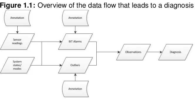
In order to apply machine learning there needs to be enough data. In this subsection the data will be explained and a number of associated challenges will be listed. The available data consists of six parts;
• Sensor readings (continuous data)
• System states (discrete data)
• System modes (discrete data)
• BIT Alarms (discrete data)
1.2. DATA CLASSIFICATION: OPEN 5
• Annotations (textual labels)
[image:15.595.148.480.188.357.2]All of these are collected periodically and are therefore stored as time series. An overview of the data flow and how this leads to a diagnosis that explains the current situation is given in Figure 1.1.
Figure 1.1: Overview of the data flow that leads to a diagnosis
1.2.1 Challenges
There are a number of challenges that result from the data described above. This subsection lists those challenges.
First of all, the dimensionality of the data is quite high, there are about 1.100 sources of continuous data such as sensors and 19.000 discrete data sources. This data is collected over time and is therefore temporal data. The sampling rate differs per sensor, some are collected every 10 seconds and some are only stored when they differ substantially from the previous reading. Given that some outliers, such as those generated during the startup sequence, are more likely to occur than others, there is also a high sample imbalance.
6 CLASSIFICATION: OPEN CHAPTER1. INTRODUCTION
annotation server is live, they are still outliers and therefore the data is by definition sparse.
Radar systems have a long lifespan of more than 30 years. This means that any fault diagnosis solution should be durable enough to keep functioning throughout the entire lifetime. This long lifetime comes with its own set of unique challenges. For one, it might happen that after 10 years a suppliers decides that a specific part will not be produced anymore, which means that it has to be replaced by another part. This means that the data that is collected is most likely different. The fault diagnosis system could handle such a change in multiple ways, one of which is through an update with a new, pre-trained, model. Another way to handle this issue is having a system that is capable of handling the change and training itself again using operator input. Since this would imply online training it is important to note that any method which uses this solution should be scalable enough to be trained now, on the currently collected data during testing, but also to train itself after 30 years worth of data has been collected.
All of this data will be collected by multiple radar systems, however all of the systems are hand-build, which means that there are slight variations in each machine. Those variations will probably make it difficult to use the trained model of one radar on the other systems. It might be possible to solve this problem through the use of techniques like Transfer Learning, however investigating this is beyond the scope of this project. Given that the market for radar systems is relatively small there will not be a lot of systems sold. Most models are sold somewhere between 10 and 100 times. This means that there will most likely not be enough data to discover the underlying structures in the data.
1.3 Research questions
The main goal of this project is to find a way to provide a diagnosis for the generated outliers automatically based on the data, which should help the operators in main-taining the radar system. This goal has lead to the following research questions:
1. To what extent can the system state be diagnosed automatically?
(a) Which techniques are available to diagnose the outliers and which are most suitable given the case described in Section 1.1 and the available data?
(b) How to assess the quality of the methods used to provide a diagnosis? (c) How do the methods selected in RQ 1.a stack up against each other
1.4. RESEARCHMETHOD CLASSIFICATION: OPEN 7
1.4 Research Method
Before trying to answer the research questions, it is important to decide on a valid research methodology for each of them. The goal of the primary research question is to find a feasible method to perform the task of diagnosing the outliers. This question will be answered through answering the sub questions. To answer RQ 1.a and RQ 1.b a literature review is performed, the result of which can be found in Chapter 3. RQ 1.c combines the two prior sub-questions to compare the found methods and find out which one is most suitable for the case of Thales as described in Section 1.2. Given that there might be (very) few labels available during the course of this project, the methods will also be compared based on a synthetic data set which has a similar dimensionality as the Thales data set, but with artificially introduced outliers and the accompanying labels.
1.5 Report organization
Chapter 2
Background
Throughout this report a large number of techniques will be mentioned that the reader is assumed to be familiar with. This chapter serves as a fallback for the cases where this assumption is incorrect. When the reader does have the background knowledge the rest of the report can be followed without reading this chapter.
2.1 Clustering methods
The goal when clustering data points is to group those data points which are more similar to each other than they are to data points in other groups. There are a large number of techniques available that try to accomplish this. This section will discuss those that form an integral part of the report.
2.1.1 K-Means
K-Means might be one of the simplest but also one of the most effective clustering methods. It tries to cluster the data points by assigning them to the nearest cluster center, often based on the Euclidian distance between the data point and the clus-ter cenclus-ter. The underlying problem is NP-hard, however when applying a heuristic algorithm it is usually possible to quickly converge to locally optimal solution. In this case the Lloyd’s algorithm is used to solve the problem. This is an iterative process that uses the following steps to cluster the data;
1. Cluster center initialization
2. Assigning data points to cluster centers
3. Updating the cluster center to be the mean of the assigned data points
4. If the means have not yet converged, return to step two
2.1. CLUSTERING METHODS CLASSIFICATION: OPEN 9
There arekcluster centers, withk being a predetermined hyper-parameter. The
k-Means algorithm has been proven to always converge to a solution. This solution might however be a local optimum [1]. One solution to this problem is to restart the algorithm several times, each with a random initialization. Another, more efficient, solution to mitigate the problem is to use a heuristic in initializing the cluster cen-ters. One such heuristic was proposed by Arthur and Vassilvitskii. They proposed to initialize the cluster centers to be generally distant from each other and proved that this leads to better results than those obtained when the initialization is done at random [2]. They dubbed this initialization strategy k-means++. The complete
algorithm is described in full detail by Hastie, Tibshirani and Friedman in their 2001 book [3].
2.1.2 Fuzzy c-Means clustering
Each clustering method has its own characteristics and one of those characteristics is whether the clusters are hard or soft. In hard clustering, each label is assigned to one cluster and one cluster only. In soft clustering on the other hand each data point has a degree of membership to a certain cluster. For example, a data point could be 70% likely to be a part of cluster A, 25% likely a member of cluster C and 5% likely a member of cluster B. Fuzzy c-Means clustering is a soft clustering variant of the previously described k-Means technique. A complete description of the algorithm is given by Dunn, who first introduced the algorithm in his 1973 paper [4].
2.1.3 Self-Organising Maps
10 CLASSIFICATION: OPEN CHAPTER 2. BACKGROUND
When the training is done, the data points are assigned to a cluster based on their BMU. When data points have the same BMU, they belong to the same cluster. SOMs are a hierarchical clustering method, which in this case means that there is more information available than just which cluster a data point belongs to. For example, if data point A belongs to the unit at(2,15)and data point B belongs to the
unit at (3,15) then the chances of the two data points are related and should
actu-ally be in the same cluster is higher than when they would be at (1,3) and (50,69)
respectively.
2.1.4 Mixture Models
A Mixture Model (MM) is a linear mixture of multiple probability distributions. The goal is to find the combination of distributions that best describe the data. Each of the distributions describes a cluster and data points are assigned to the distribution that has the highest probability for their value. Even though this sounds good in the-ory it does require that the parameters of each distribution are estimated. Since it is not clear which of the data points belong to which distribution it is difficult to properly estimate the values. This is where the Expectation Maximization (EM) algorithm comes in. This algorithm, which consists of an expectation and a maximization step, iteratively estimates the parameters to achieve the maximum likelihood. In his 2006 book Bishop gives a more detailed description of MMs [6].
2.1.5 Support Vector Machines
2.1. CLUSTERING METHODS CLASSIFICATION: OPEN 11
of these two methods proofed most effective [11], [12].
Even though SVMs are traditionally supervised learning algorithms, it is possible to also include unlabelled instances. This is done through a Transductive Support Vector Machine (TSVM). TSVMs calculate the maximum margin solution, while si-multaneously finding the most suitable label for the unlabeled instances [13].
2.1.6 Subspace clustering
When working with high-dimensional data there are often subspace in the data that can be identified and utilised to perform clustering. Subspace Clustering (SC) as this is called is a group of clustering techniques. This subset of clustering algorithms tries to cluster the data points based on a limited number of subspaces, so cluster
aand b might only exist in the combination of dimension1and 2, whereas cluster c
only exists in dimensions3and 4. In order properly differentiate these clusters they
should be looked at in their respective dimensions. More details on this technique and the exact implementation can be found in Parsons’ 2004 book [14].
2.1.7 Semi-supervised clustering
In unsupervised learning the algorithms do not use any information about the un-derlying data to create clusters, whereas supervised learning requires all of the data to be labelled in order to train. A middle ground here is semi-supervised learning, which uses side information about the data to create a more accurate clustering. Semi-Supervised learning arose in the 60s when the concept of self-learning algo-rithms was introduced by Scudder. The technique really started to take of in the 70s however when researchers began to incorporate unlabelled data whilst training mixture models [15]. According to Chapelle, Schlkopf, and Zien [15] the term semi-supervised learning itself was first introduced in the context of classification by Merz et al. [16].
12 CLASSIFICATION: OPEN CHAPTER 2. BACKGROUND
that they must be linked in the same cluster, whereas a C-L means that the sam-ples must be in a different cluster. The label based method is more informative, but the constraint based technique is a more generally applicable. It is possible to use labels as the basis in a constraint based setting, but not the other way around [17].
2.2 Dimensionality Reduction
When the data consists of a large number of dimensions it might be required to reduce the dimensionality before using the data for applications such as clustering. This is because relevant patterns are likely to be overshadowed by meaningless data from other dimensions. The general goal of dimensionality reduction is to map the data to a lower dimensional subspace without losing information. There are multiple methods that try to achieve this goal. This sections tries to give some background on three that are important to this report.
2.2.1 Principal Component Analysis
Principal Component Analysis (PCA) is a linear transformation algorithm. The goal of the algorithm is to find the directions (lines) of maximum variance. It iteratively starts by finding the one with the maximum variance and is called the first compo-nent. It then tries to find another component, with the second highest variance, that has to be mutually orthogonal to the others. The first direction is called the first prin-cipal component, the second is called the second prinprin-cipal component, etc. Each component has an eigenvalue associated with it, that indicates the amount of vari-ance that it is responsible for. This means that those components with the lowest eigenvalue are also the ones that could best be thrown away. There are multiple techniques to find those components, however the most popular one is Singular Value Decomposition (SVD). More details on this method can be found in Bishop (2006) [6].
2.2.2 Stacked Auto-Encoder
2.2. DIMENSIONALITYREDUCTION CLASSIFICATION: OPEN 13
lower dimensional representation of the data. A more detailed explanation can be found in Aggarwal’s 2018 book [18].
2.2.3 Deep Belief Network
Chapter 3
Literature review
As was established in the Chapter 1, the goal of this report is to find a method to automatically explain the system’s behaviour, either through a literature review or by creating a novel method. In this section a literature review will be performed to do so. With the advent of cheaper sensors and storage, the field of monitoring equipment and detecting and classifying faults has become an increasingly popular one. This is often done by inferring the system state from the relevant sensor readings. In the literature this is often called Fault Detection and Diagnosis (FDD). According to the Scopus database a total of 3.397 articles or conference papers have been published on the topic of Fault Diagnosis in 2018 alone. Thales already has a system in place to detect the outliers. However it is not yet possible to diagnose those outliers.
3.1 Fault diagnosis
Isermann identified two methods of performing fault diagnosis [19], data-driven meth-ods and reasoning based methmeth-ods. Of these two methmeth-ods the latter mainly relies on a-priori knowledge of the system, whereas the prior is a data driven approach. Given the high complexity of the radar system it is infeasible to encode all the ex-pert knowledge required to diagnose every possible fault into the system. Another complicating factor with the reasoning based approach is that there is most likely not enough expert knowledge to determine every possible fault beforehand. Therefore this research will focus on the data-driven diagnosis method. In order to review the literature available on data-driven fault diagnosis a structured literature review was performed. This search was performed on the Scopus database, with the goal of finding all articles and conference papers related to clustering or classification in the area of fault diagnosis. Since this yielded over 5.500 results, the search was limited to work published after 2016. This resulted in the following search query and a total of 1.280 results at the time of writing (the 13th of March 2019).
3.1. FAULT DIAGNOSIS CLASSIFICATION: OPEN 15
TITLE-ABS-KEY (fault AND diagnosis) AND (TITLE-ABS-KEY(classification) OR
TITLE-ABS-KEY(clustering)) AND (DOCTYPE(ar OR cp) AND PUBYEAR > 2016)
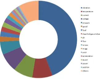
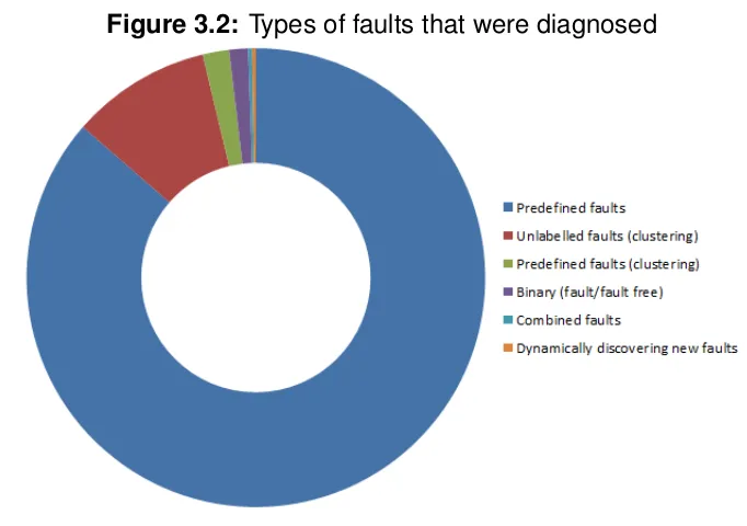
[image:25.595.151.475.420.675.2]The results of this search were then scanned manually to filter out work that did not concern itself with fault diagnosis in machines or electrical equipment, which brought the number of papers down to 404. Those papers were then categorized based on the techniques used, their application area, the type of data, the method through which the diagnosis was created and whether they are supervised, unsuper-vised or semi-superunsuper-vised. The complete categorization can be found in Appendix A. The doughnut charts in Fig. 3.1 and Fig 3.2 are generated based on this categoriza-tion. From those charts it becomes apparent that the most popular type of data is vibration data. This was used in almost half of all cases. It is also clear that the most popular type of fault diagnosis is through predefined faults. In those cases there is a set of fault classes and the algorithm assigns one of those to a reading. The second most used method is by clustering the readings and not assigning descriptions at all.
Figure 3.1: Data types used for fault diagnosis
16 CLASSIFICATION: OPEN CHAPTER3. LITERATURE REVIEW
Figure 3.2: Types of faults that were diagnosed
3.1.1 Spacecraft
3.1. FAULT DIAGNOSIS CLASSIFICATION: OPEN 17
whereas the training time did increase substantially [20].
3.1.2 Power systems
Wu et al. designed a fault diagnosis system for power systems where they tried to differentiate between three fault modes. This diagnosis is done using a classification algorithm which sees the fault modes as classes. The test set used by Wu et al. is smaller than the one used by Li et al., this set has nine features and 200 samples. The classification between the three classes was done using a one-vs-all SVM clas-sifier. All of these classifiers are trained twice, once for the voltage data and once for the current data. This leads to two sets of three classifiers. If the classifications of those two are inconsistent with each other the results will then be processed by the fusion step. This fusion step uses the Dempster-Shafer (D-S) evidence theory to decide which of the two classifications to use. However, when applying SVM there are two parameters that need to be determined beforehand, the penalty factor (C)
and the kernel parameter (γ). Since there is no way to mathematically find the
opti-mal value for these parameters, there is no straightforward method of finding a good value for them. The way Wu et al. solved this problem was by a grid search of all possible values. However, with two real-valued parameters that are not limited the possible combination are endless. Therefore they used a Genetic Algorithm (GA) to speed the process up and come up with a good value within a reasonable amount of time. A GA is a metaheuristic that draws from the Darwinistic principles of nature to iteratively improve the solution. To prevent overfitting k-fold cross validation was
applied in this grid search. The accuracy of the proposed classifier were compared to those of a standard SVM and a SVM that was optimized using Particle Swarm Optimization (PSO). This comparison showed that the GA SVM D-S algorithm per-formed better than the two opposing approaches [21].
3.1.3 Bearings
18 CLASSIFICATION: OPEN CHAPTER3. LITERATURE REVIEW
main problems with GG clustering for their application, it counts all samples equally and it has difficulty in selecting the optimal number of clusters. To overcome the former of those issues they incorporated the Non-parametric Weighted Feature Ex-traction (NWFE) method. This technique assigns weights to the different samples, more effectively use the local information. To determine the number of clusters, the PBMF clustering validity index is used. This index, which looks to balance out intra-class compactness and inter-intra-class separability, provides a score given a number of clusters, the higher this value, the better suited the clustering. To determine the number of clusterK the proposed Adaptive Non-parametric Weighted-feature
Gath-Geva (ANWGG) iteratively increases theKby one, until it reachesKmaxwhich is set
to √N, withN being the number of samples. To do dimensionality reduction Zhao
and Jia also incorporated a DBN. The proposed setup was tested on three different cases, all of which concerned vibration data from a bearing test setup with a num-ber of labelled faults. The algorithm was compared to GG clustering, Fuzzy c-means clustering and GustafsonKessel (GK) clustering based on four criteria, the PBMF in-dex, the Partition Coefficient (PC), Classification Entropy (CE) and the error rate. The first three are indicators of clustering quality and are calculated solely based on the cluster structure, whereas the error rate is calculated using the labelled sam-ples. The clusters are given labels during the training phase based on the largest membership degree, that is to say, the cluster label is determined by which class is the most common in the cluster. Based on this measure it became clear that the proposed setup performed better than the alternatives, albeit with a slightly higher runtime [22].
3.1.4 General datasets
Hou and Zhang developed a clustering methodology which they proposed as a can-didate for fault diagnosis, but did not test in this situation directly. However they took a slightly different approach. Instead of using a density based clustering method, which uses the distance to the cluster center they applied the Dominant Set algo-rithm, which determines the clustering based on the pairwise similarity between two points. The main benefit of this is that it allows for non circular clusters. Another ben-efit is that there are no parameters that need to be tuned. The test case that was used to validate the proposed methodology on a variety of public datasets which are published with the goal of providing researchers with a dataset to test their al-gorithm against. The Dominant Set based alal-gorithm was compared to traditionally popular clustering methodologies such as Affinity Propagation (AP), k-means and
In-3.2. PERFORMANCE METRICS CLASSIFICATION: OPEN 19
formation (NMI) index, which both compare the results of the clustering to the ground truth to come up with a score of the clustering performance. This test showed mixed signals, the proposed algorithm performed better than the rivals on some datasets but worse on others [23].
3.2 Performance metrics
The metric that is used to measure the performance of a clustering algorithm is an important decision as it defines what is considered ”good”. When class labels are available and the algorithm in question is capable of assigning class labels the most used measure of quality is accuracy, which is defined as the percentage of correctly classified samples. This metric is used among others by the first two papers de-scribed above. However, when no ground truth is available or when the algorithm is not capable of assigning class labels, another way of measuring the quality should be found. This has proven to be a challenging task, mainly due to the fact that there is no knowledge of the underlying structure of the data. There are generally speaking three types of criteria by which to judge the performance of clustering al-gorithms, external-, internal-, and relative criteria [24]. External criteria judge the resulting clusters based on a priori knowledge of the structure of the data. This can manifest itself in different forms, though the most common one is labelled data. Although such criteria would often lead to the most reliable results, it is often im-possible to use them outside a controlled test environment. Internal criteria on the other hand only use the data itself to rank the result. The last option compares the resulting clusters to other clusters, generated by the same algorithm. Since there is no knowledge of the underlying distribution of the data and the goal of this study is to compare different algorithms, their performance will be measured based on in-ternal criteria. This type of measurements usually focuses on two main properties, inter-cluster separability and intra-cluster density [25].
20 CLASSIFICATION: OPEN CHAPTER3. LITERATURE REVIEW
X The data set
N The number of samples in data setX C The set of all clusters
ck The centroid of clusterck, defined as the mean vector of the cluster:
ck = |c1
k| P
xi∈Ckxi
X The centroid of data setX, defined as the mean vector of the data
set: X = N1 P
xi∈Xxi
de(xi, xj) The euclidean distance between two pointsxi andxj
Silhouette index
The silhouette index measures for each sample how similar it is to its own cluster based on the distance between the sample and the other samples in the same cluster (a(xi, ck)) and what the distance is to the closest cluster that it is not part
of (b(xi, ck)) [26]. The equation below shows the mathematical definition as it was
used by Arbelaitz et al. [24].
Sil(C) = 1
N X
ck∈C X
xi∈ck
b(xi, ck)−a(xi, ck
max b(xi, ck),a(xi, ck)
(3.1)
Where:
a(xi, ck) =
1
|ck|
X
xj∈ck
de(xi, xj),
b(xi, ck) = min cl∈C\ck
1
|cl|
X
xj∈cl
de(xi, xj)
!
.
Davies-Bouldin index
The Davies-Bouldin index measures the same qualities as the Silhouette index, but does so using the cluster centroids instead. The density is measured based on the distance from the sample to the cluster centroid and the separability is calculated as the distance from the sample to the nearest cluster centroid that it is not part of [27]. This is defined as follows by Arbelaitz et al. [24].
DB(C) = 1
K X
ck∈C max
cl∈C\ck
S(ck) +S(cl)
de(ck, cl)
!
(3.2)
Where:
S(ck) =
1
|ck|
X
xi∈ck
3.2. PERFORMANCE METRICS CLASSIFICATION: OPEN 21
Calinski-Harabasz index
In the Calinski-Harabasz index the separability is not determined based on the in-dividual samples but instead on the distance from the cluster centroid to the global centroid. Just as in the Davies-Bouldin index the density is measured by taking the distance from each sample in the cluster to the cluster centroid [28]. The mathemat-ical definition in Equation 3.3 is courtesy of Arbelaitz et al. [24].
CH(C) = N −K
K−1
P
ck∈C|ck|de(ck, X) P
ck∈C P
xi∈ckde(xi, ck)
(3.3)
3.2.1 Supervised metrics
To evaluate the results during training and on the real data set, in other words, when no truth data is available, measures such as the ones above need to be used. However when the actual labels are known it is possible to use other, more informa-tive, measures. There are a number of often used validity measures for supervised classification tasks. These metrics are based on the results from a confusion ta-ble. These results include theTrue Positives(TP) (the number of samples that were
correctly classified as positive), the True Negatives (TN) (the number of samples
that were correctly classified as negative), the False Positives (FP) (the number of
samples that were wrongly classified as positive) and theFalse Negatives(FN) (the
number of samples that were wrongly classified as negative).
Sokolova and Lapalma performed a systematic analysis of classification perfor-mance measures for, among others, multi-class classification [29]. The measures that are proposed are average accuracy, error rate, precisionµ, recallµ, F-Scoreµ,
precisionM, recallM and F-scoreM. For the precise definition please refer to [29]. The
measures they propose for multi-class classification are the same as the ones for binary classification, with the exception that they are averaged for multiple classes. The averaging can be done in two ways; macro averaging (M), where the sum of
the measures is averaged, and micro averaging (µ), where the sums of the different
22 CLASSIFICATION: OPEN CHAPTER3. LITERATURE REVIEW
3.3 Techniques
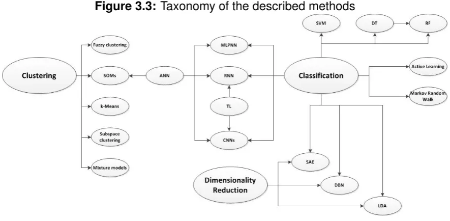
[image:32.595.63.506.228.445.2]The goal of this section is to provide an overview of all the methods that have been applied to fault diagnosis over the last two years and to identify other, high potential methods. This is done using the same search query that was used in Section 3.1. A taxonomy of all the methods that are discussed in this section, can be found in Figure 3.3.
Figure 3.3: Taxonomy of the described methods
3.3.1 Fault Diagnosis
This section will list the methods that were found in the fault diagnosis literature. The methods are divided into two groups, classification and clustering.
Classification
One of the most popular methods to perform fault diagnosis is the SVM. In total, 102 of the reviewed papers used some form of SVM. Naturally there are differences between the different implementation such as the use of different kernel functions, e.g. RBF [7], [8] or the PUFK [9]. Another difference between the implementations is how many classes they can differentiate. Traditional SVMs can only differentiate between two classes. When doing multi-class classification instead a choice has to be made between the OAA and the OAO strategy. In the literature the latter of these two methods proofed most effective [11], [12]. Lou et al. used TSVMs to include unlabeled instances as well while doing fault diagnosis [30].
3.3. TECHNIQUES CLASSIFICATION: OPEN 23
DT consists of a number of nodes. Each node in a DT splits the dataset based on one attribute. This is done until only the instances of one class remain. In total 18 of the reviewed papers used DTs to perform classification. One of these papers com-bined DTs with the unsupervisedk-means algorithm, which will be described later
on, to create a semi-supervised classifier. In their approach two models are trained, one DT based on the labeled data and onek-means based on the unlabelled data.
These two models are then combined to classify new instances [31]. A benefit of DTs over most other methods described in this section is it’s explainability. Since a DT is only a combination of decisions steps, it is easy to explain how a certain decision was made.
RF is an ensemble learning technique that combines multiple DTs to get a better classification result than with just one DT. In a RF each DT only has access to a random subset of features and training samples, which should prevent issues such as overfitting. RFs are used by 11 of the reviewed papers, however all of these used it in a supervised fashion.
A technique that has seen more and more widespread use in recent years are Arti-ficial Neural Networks (ANN). ANNs are popular because of their widespread appli-cability, they have been used for a lot of things, including image classification, sales forecasting and fault diagnosis. There are different implementations of this idea, the simplest of which is probably an Feed Forward Neural Network (FFNN) with only an input and an output layer. When more layers are added, this forms a Multi-Layer Perceptron Neural Network (MLPNN). A MLPNN has one or more hidden layers be-tween the input and the output layer where calculations are performed. The training of MLPNNs is usually performed in a two phased fashion, a forward phase and a backward phase. The forward phase is used to calculate the loss function and the
backward phase is used to update the weights. This technique is calledback propa-gation[18]. Since 2016 the MLPNN has been applied to fault diagnosis a total of 29
times, sometimes on its own, sometimes in cooperation with other algorithms, such as DT [32] or the Hidden Markov Model (HMM) [33].
24 CLASSIFICATION: OPEN CHAPTER3. LITERATURE REVIEW
used five times in the field of fault diagnosis, of which one time in conjunction with a Convolutional Neural Network (CNN) [34].
The origin of CNNs lies in the field of image recognition, where it has proven to be one of the most successful Neural Network (NN) architectures. Based on this success CNNs have been used in all kinds of fields, including object detection and text processing. Since 2016 CNNs have been applied 28 times to fault diagno-sis problems, sometimes in conjunction with other algorithms such as DBN [35] or HMMs [36].
One of the issues with CNNs is that it takes a lot of labelled data to train the net-work. One solution to this is to use Transfer Learning (TL). TL is a technique that uses information from a previous task to speed up training on this task. It requires another neural network that is trained on different, but similar data. For example if you want to train a NN that identifies cows you could use a NN that classifies cats and dogs as a basis. You then delete the existing loss-layer while keeping the rest of the network and train it again on the, smaller, set of labelled cow images. This technique is not only used for CNNs but also for example for RNNs [18]. It has been applied to fault diagnosis a number of times during the last years, among others by Hasan et al. [37] and Wang and Wu [38]. DBNs have also been applied to fault diag-noses. When applied to classification, which is their main task in the fault diagnosis literature, the DBNs are mainly used in a supervised manner [39]–[41]. There have however also been papers that applied DBNs to fault diagnosis in a semi-supervised or unsupervised manner, although this is mainly in the role of a dimensionality reduc-tion algorithm. Zhao and Jia used a fuzzy clustering method for the semi-supervised clustering and a DBN to perform dimensionality reduction in the context of rotating machinery [22]. The same combination was also applied by Xu et al., though in their case the clustering was performed completely unsupervised and in the context of roller bearings [42].
AEs originate in the field of dimensionality reduction and are an unsupervised neural network that try to find a, lower dimensional, encoding for the data. SAEs or their rel-ative the Stacked Denoising Auto Encoder (SDAE) [43] have been used in the fault diagnosis literature to do both classification, in conjunction with another layer or al-gorithms such as a SVM [44] or a softmax classifier [45], [46] or semi-supervised clustering, where the data is first clustered unsupervised and the clusters are then improved using a small set of labelled data [47].
Clustering
3.3. TECHNIQUES CLASSIFICATION: OPEN 25
but instead uses competitive learning [18]. Like AEs, SOMs are typically used for dimensionality reduction, but can also be used for clustering. This was done, among others, in the field of fault diagnosis by Blanco et al. [48] and eight others.
Even though neural networks are widely popular nowadays there are also other tech-nologies that offer promising results. One of the most popular of these is k-means clustering and its supervised relative k-NN classification. K-means is used a total of five times to perform fault diagnosis [49], often in conjunction with other methods such as HMMs [50] or SVMs [51].
The k-NN algorithm is about as popular when it comes to fault classification, seeing as it was applied six times since 2016.
Another popular clustering technique is fuzzy clustering. The main difference be-tween fuzzy clustering and traditional or ”hard” clustering methods such as k-means is that fuzzy clustering allows data points to belong to multiple clusters. One of the most popular variants of fuzzy clustering is fuzzy c-means clustering. This tech-nique was first introduced by Dunn in 1973 [4] and is highly similar to the traditional k-means clustering. It was successfully applied to fault diagnosis [52], [53] a total of 17 times in different fields, including roller bearings [54] and wind turbines [55]. When working with high-dimensional data there are often subspace in the data that can be identified and utilised to perform clustering. SC uses these subspaces to identify clusters in the data. SC has been applied to fault diagnosis in bearings by Gao et al. [56].
3.3.2 Classification in high-dimensional sparse data
In the previous section it became apparent that most of the techniques that were re-cently used in fault diagnosis are based on classification or clustering algorithms. In order to find ways to expand this body of methods a second search was performed. This search focused on the type of data as it was described in Section 1.2, namely sparse, high-dimensional data, with a small and incomplete set of labels, although the labels are not explicitly taken into account in the search query, which looks as follows:
(ab:(classification) OR ab:(clustering) OR ab:(categorization) OR ab:(grouping))
AND (ab:(sparse) OR ab:(sporadic) OR ab:(infrequent) OR ab:(scattered)) AND
(ab:(high-dimensionality) OR ab:(high dimensionality))
26 CLASSIFICATION: OPEN CHAPTER3. LITERATURE REVIEW
results were categorized based on four characteristics, the main application (dimen-sionality reduction, classification, regression or outlier detection), the techniques that were used, the application field and whether they were supervised, unsuper-vised or semi-superunsuper-vised. On the results snowballing was performed, up to three levels deep, with increasing scrutinization. The complete result can be found in Ap-pendix B.
A large portion of the literature focused on dimensionality reduction, however there are a number of interesting algorithms that have not been used for fault recognition yet. Given that the data set has a (very) limited amount of labels, only unsupervised and semi-supervised techniques will be considered.
Linear Discriminant Analysis (LDA) is a technique that is mainly used for supervised dimensionality reduction and classification. Zhoa et al. used this technique in a semi-supervised manner to perform image recognition by using a process called la-bel propagation, where the lala-bels are propagated to the unlala-belled instances. Those new labels are called ’soft labels’ [57]. To make sure that LDA has not been used in fault diagnosis yet, a search was done. This turned up a total of 82 results where LDA was used for fault diagnosis, including for Re-useable Launch Vehicles [58] and motor bearings [59], meaning that the use of LDA in fault diagnosis is not new. Another clustering algorithm that came up in the search is the MM. MMs try to sep-arate the clusters based on a probability distribution, for which the parameters are approximated using a technique called EM [60], [61]. Even though it did not appear in the search for papers after 2016, MMs have been used to perform fault diagnosis before, among others Luo and Liang [62] and by Sun, Li and Wen [63].
One way of doing semi-supervised learning is through TL, a technique that was explained in Section 3.1. Self-taught learning is another technique that works in a similar manner. However, self-taught learning does not assume that the additional, unlabelled, samples have the same distribution or class labels [64]. This techniques has not been applied to fault diagnosis yet.
Although they have delivered great results in the past, unsupervised learning meth-ods and techniques like TL might not always be up to the task. In that case a supervised algorithm could be required. However, it is usually still too expensive to label all the data. This is where Active Learning (AL) comes in. AL is a supervised algorithm that selects instances from the pool of unlabelled samples and asks an ”oracle”, usually a human annotator, to label them. This limits the amount of work that the oracle needs to perform, while still being able to train a supervised classi-fier [65], [66].
3.4. SUMMARY CLASSIFICATION: OPEN 27
the random walk and the parameters are optimized using the EM algorithm. Like self-taught learning, no papers could be found in the Scopus database where this tactic was applied to the field of fault diagnosis.
3.4 Summary
The literature review on machine learning models in fault diagnosis has resulted in a lot of promising results. A large number of clustering and classification algorithms have already been applied successfully to this field. However there are still a number of shortcomings when it comes to the specific case of Thales as it was described in Chapter 1.
The main problem here lies in the type of data that was used as an input for the di-agnosis. In the reviewed literature it often concerned either vibration data or image data. In the case of Thales the data consists of a large number of sensor measure-ments, which makes for a very different situation. A large number of the reviewed papers also assumed that there were a limited number of fault classes or that all data is labelled. This is not the case here. The majority of the data is unlabelled, which makes is infeasible to apply supervised classifiers. This means that only a few of the proposed algorithms can be applied to Thales’ problem as only semi-supervised and unsupervised algorithms qualify. Out of the algorithms described in Section 3.1 the following algorithms are capable of semi-supervised or unsupervised learning: TSVMs, k-means clustering, SOMs, fuzzy c-means clustering and SC. However most of these, with the exception of subspace clustering, will not perform well on high-dimensional data without some sort of preprocessing such as feature transfor-mation or feature extraction. In the literature the process of feature extraction was often done using DBNs or SAEs.
In Section 3.3.2 five methods were identified that have been applied successfully to classification or clustering in high-dimensional data with few or no labels. Two of these, LDA with label propagation and MM have been applied successfully to fault diagnosis, albeit before 2017. In the literature there was no example found where the three remaining methods, self-taught learning, AL and the MRW were applied to fault diagnosis.
28 CLASSIFICATION: OPEN CHAPTER3. LITERATURE REVIEW
methods are deemed infeasible in the situation of Thales during the course of this project, however they would warrant future research. Another method that requires extra data is AL. This method needs an oracle that can provide feedback. Given that the time and availability of the oracles is limited, it would be uncertain if it is possible to implement and test this method within the course of this project. Given this constraint, AL will not be implemented, however it is advised that this method is researched further in the future.
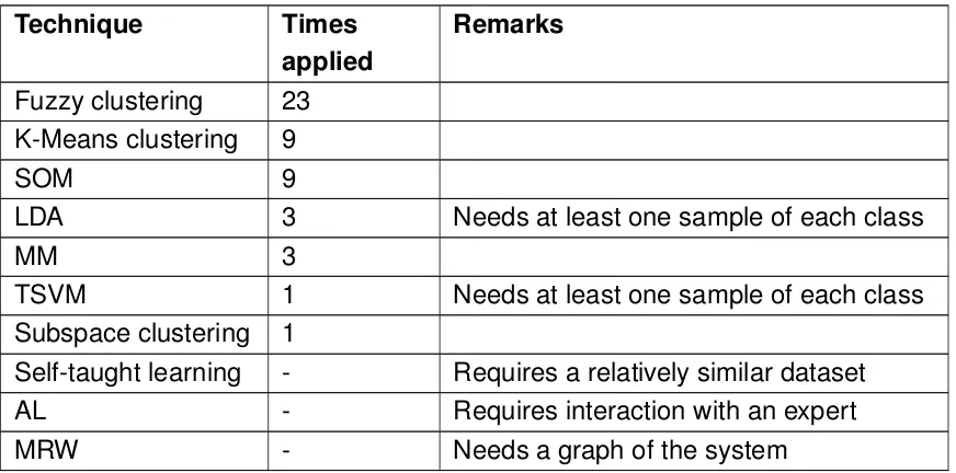
Based on the background set out in the previous section and popularity in the fault diagnosis literature the following methods were selected: fuzzy clustering, k-Means clustering and SOMs.
Another area of research that showed some promising results in the literature but was not very popular was semi-supervised learning. In order to test whether this is indeed of added value, a semi-supervised method will also be tested. In order to easily compare this approach to the unsupervised methods, a semi-supervised variant of the SOM will be used.
The performance of those techniques will be compared on the Thales dataset and an artificial dataset, which will be described later in Section 4.1. Parameter estima-tion will be performed using a Genetic Algorithm as was proposed by, among others, by Wu et al. [21]. Finally, every method will be tested without and with dimension-ality reduction performed by a DBN, which in the research of Li et al. turned out to outperform PCA and SAE [20].
Technique Times applied
Remarks
Fuzzy clustering 23
K-Means clustering 9
SOM 9
LDA 3 Needs at least one sample of each class
MM 3
TSVM 1 Needs at least one sample of each class
Subspace clustering 1
Self-taught learning - Requires a relatively similar dataset
AL - Requires interaction with an expert
[image:38.595.68.504.457.673.2]MRW - Needs a graph of the system
Chapter 4
Methodology
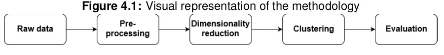
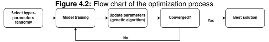
[image:39.595.89.539.559.615.2]A valid research methodology is the basis of every good piece of research. Based on the conclusions from the previous section, the methodology that was proposed in Section 1.4 can be extended. RQ1.a and RQ1.b have already been answered in the previous section through a literature review. The one remaining question is RQ1.c. This question will be answered in a data-driven fashion, as is common in the related literature described above. To evaluate the three algorithms that were selected, k-Means clustering, fuzzy c-Means clustering and SOMs, they will be tested on multiple data sets. The evaluation is done in three steps, (1) pre-processing, (2) dimensionality reduction, (3) clustering and (4) evaluation. Figure 4.1 provides a visual representation of these steps, which will be described in more detail in the sections below. During steps two and three there are a number of hyper-parameters that need to be determined. The search spaces in which those values can lie are already described in each respective subsection. The manner in which the search is performed is described at the end of this chapter in Section 4.6. Before going into detail on the steps themselves, the data sets will be discussed shortly.
Figure 4.1: Visual representation of the methodology
4.1 Data
As was mentioned before, the different methods will be tested on three synthetic data sets and one real data set. The synthetic data sets are created by domain experts with the goal to be similar to the real data set. In this case synthetic data sets are used because it is difficult and expensive to get a real data set. Using synthetic data makes it possible to quickly test the performance of the algorithms in
30 CLASSIFICATION: OPEN CHAPTER4. METHODOLOGY
a controlled environment. Since it is possible to control the number of dimensions, it is also easier to visualize the data, which helps to get a quicker insight into the data. The real data set covers a period of five months and is annotated manually by a domain expert. This was done through a visual inspection of the time series. Since domain experts are mere humans, it is possible that this annotation is not 100% correct, however it should serve as a good benchmark for the algorithms. More details on these data sets are provided in Appendix C.
4.2 (1) Pre-processing
The data set consists of a large number of sensor reading that all have their own characteristics. If they are compared without any pre-processing, based on the eu-clidean distance, observations that have a different magnitude will have a dispropor-tionate effect on the results. Therefore some data pre-processing is required. The features will be scaled using a technique called z-normalization, where the mean of the feature is subtracted from the data and it is then divided by its variance. The exact formula isXi = µXσ−Xi
X with X being a feature vector, ibeing a sample in that
feature vector, µX being the mean of the feature and σX being the standard
devi-ation. As a further pre-processing step, all alarms will be removed from the data, since according to Thales’ domain experts most of the variables are merely an alarm raised when another reading crosses a certain threshold. Thus this data is already derived from other observations and will be disregarded.
4.3 (2) Dimensionality reduction
As was described in Section 3.4, the dimensionality reduction will be performed by a DBN. Each of the clustering methods will be tested both with and without dimension-ality reduction, to get a clear view of its influence on the results. When implementing a DBN there are a number of hyper-parameters, most of which are found in most neural networks. These includes the activation function, the learning rate, the num-ber of epochs, the batch size and the structure of the network (i.e. the numnum-ber of hidden layers and the number of neurons per layer). To determine the size of the search space the recommendations of Bengio for hyper-parameters in neural net-works will be used [68]. As activation function only the ReLu function will be used, since this is one of the few activation functions that do not suffer from the vanish-ing gradient problem [69]. Accordvanish-ing to Bengio the optimal learnvanish-ing rate for cases where the input is mapped to a range of (0,1), lies in the range (10−6,1]. Since a
4.4. (3) CLUSTERING CLASSIFICATION: OPEN 31
it is added to an initial value of0.1, the values in the range will increase with10% of
their value at each step (i.e. from 0.01 to 0.011 and from 0.1 tot 0.11). Since there
is no ”rule of thumb” available for the number of epochs, the search range will be limited at the interval(5,250), with a uniform distribution over the interval. This range
is chosen to get a good overview of all values, while still maintaining a reasonable training time. The batch size is an important hyper parameter to optimize as it deter-mines how many times per epoch the parameters are updated. There are generally speaking three options, a stochastic, or online, training where the batch size is one (i.e. there are no batches), a mini-batch, where the data set is divided into multiple batches which are all larger than one and ”normal” batch training where all samples are entered in one batch. In the case of a large training set, the batch method is infeasible as it will most likely have trouble converging or at least be very slow. In accordance with the recommendation from Bengio the batch size will be searched over the interval (1,200). The network will be tested with zero to five hidden layers
and 25 to 200 neurons per layer.
4.4 (3) Clustering
As was concluded in the previous chapter, a total of three clustering methods will be compared to each other on three synthetic data sets and one real data set. This section describes the algorithms that are compared to each other.
4.4.1 k-Means Clustering
The k-Means clustering algorithm is a popular algorithm to partition a data set into
k different clusters. The details of the algorithm were described in 2.1.1. As an
initialization schema k-Means++ will be used. The k-means algorithm is relatively
simple, which means that there is only one parameter that needs to be estimated, namelyk. This parameter determines the number of clusters that the data set needs
32 CLASSIFICATION: OPEN CHAPTER4. METHODOLOGY
4.4.2 Fuzzy Clustering
Fuzzy clustering was implemented using the Fuzzy c-Means algorithm. This tech-nique, which is related to the k-Means algorithm which was described in the previous section, is used because of its widespread usage in the related works. The imple-mentation is based on the one put forward by Bezdek, Ehrlich and Full in their 1982 paper [70]. Since fuzzy clustering is a soft clustering methodology, samples are not automatically assigned one specific cluster, but instead have a membership to each cluster. In order to be able to compare the results from the fuzzy clustering to that of the other clustering methodologies, the data points are later assigned to the clus-ter with the highest membership factor. In fuzzy c-Means clusclus-tering there is also just one hyper parameter that may be tuned, namely the number of cluster centers. Given that this is the same parameter as the one that needs to be tuned in k-Means clustering, the search space will be the same as well.
4.4.3 Self-Organizing Maps
The concept of a SOM was first introduced by Kohonen in 1982 [5]. In this case the SOM is used as an unsupervised clustering algorithm, however it can also be used for dimensionality reduction. SOMs revolve around BMUs. A SOM consists of a map of nodes. In this map the different units are assigned weights, which are then updated based on the samples closest to them (i.e. the samples for which the unit is the best match). The clustering is done based on these BMUs. Each BMU represents a cluster and the samples are assigned to the BMU, and thereby to the cluster, that best matches them. In order to train a SOM there are four parameters that need to be set, the number of epochs, the learning rate and the width and the height of the map. For the number of epochs and the learning rate the same search space is used as for the DBN. The height and width of the network is, among other things, dependent on the number of samples and the number of clusters in the data. The width and height together determine the size of the map (size=width∗height).
The lower bound for the size of the map is the number of distinct clusters. In this case the lower bound is given by the number of distinct, known, class labels (see Section 4.4.1 for more details). The upper bound is given by the number of samples in the entire data set times two.
4.4.4 Constraint-Based Semi-Supervised Self-Organizing Map
substan-4.5. (4) EVALUATION CLASSIFICATION: OPEN 33
tial benefit. Some background on semi-supervised clustering can be found in Sec-tion 2.1.7. Since the constraint-based variant of semi-supervised clustering is more versatile than its label-based counterpart the learning will be performed using con-straints. This offers more possibilities when it comes to gathering user input, such as asking the question ”Do these two samples belong to the same fault?”, which makes it easier for the operator to provide input. In the Scopus database only one paper could be found that worked on incorporating constraints into the SOM. Allahyara, Sadoghi and Haratia did worked on such a variant, however they focused solely on an online variant, whereas the focus of this report is on offline learning [71]. There-fore this section proposes a new extension to the SOM to incorporate constraints while doing offline learning. The details of this implementation are described in Ap-pendix D.
4.5 (4) Evaluation
Based on the results of the literature review performed in Section 3.2 two metrics are selected to evaluate the results of the clustering, one that does not require truth data and one that does.
From the definitions given in Section 3.2, it shows that the Davies-Bouldin index and the Calinski-Harabasz index are both calculated based on the cluster centroids, whereas the Silhoutte index is calculated by taking the distance between each sam-ple. One of the main pitfalls of the centroid based methods is that they, due to their nature, favour circular clusters. Since this is an assumption that can not be made at this point, the Silhoutte index will be used when there is no truth data available, even though it is a more computationally intensive measure.
When selecting a supervised quality metric an important point to keep in mind here is that the data is highly imbalanced. When using macro-averaging, all classes are weighted equally, whereas in micro-averaging the classes with more samples are favoured. Given Thales’ imbalanced data set, macro-averaging will be used. The imbalanced data set also implies that some measures are more suitable than others. For example, if an event occurs only three times in a data set of 200 samples and the classifier gives none of the samples this label, it will still have an accuracy of
98.5%. Therefore measures such as recall and precision are more suitable. In this
case the F-score will be used. This score is the harmonic mean of the recall and the precision and provides a comprehensive representation of performance, without suffering the effects of an unbalanced data set.