Large scale drift and Rossby wave turbulence

warwick.ac.uk/lib-publications

Original citation:

Harper, Katie L. and Nazarenko, Sergey. (2016) Large-scale drift and Rossby wave turbulence.

New Journal of Physics, 18. 085008

Permanent WRAP URL:

http://wrap.warwick.ac.uk/80452

Copyright and reuse:

The Warwick Research Archive Portal (WRAP) makes this work of researchers of the

University of Warwick available open access under the following conditions.

This article is made available under the Creative Commons Attribution 3.0 (CC BY 3.0) license

and may be reused according to the conditions of the license. For more details see:

http://creativecommons.org/licenses/by/3.0/

A note on versions:

The version presented in WRAP is the published version, or, version of record, and may be

cited as it appears here.

Warwick Mathematics Institute, University of Warwick, Gibbet Hill Road, Coventry, CV4 7AL, UK

E-mail:Katie.Harper@warwick.ac.ukandS.V.Nazarenko@warwick.ac.uk

Keywords:Rossby waves, drift waves, turbulence, energy cascade, zonal jets

Abstract

We study drift

/

Rossby wave turbulence described by the large-scale limit of the Charney–Hasegawa–

Mima equation. We de

fi

ne the zonal and meridional regions as

Z

≔ {

k

:

∣ ∣

k

>

3

k

}

and

<

≔ {

∣ ∣

}

M

k

:

k

3

k

respectively, where

k

=

(

k

,

k

)

is in a plane perpendicular to the magnetic

fi

eld such that

k

is along the isopycnals and

k

is along the plasma density gradient. We prove that the

only types of resonant triads allowed are

M

«

M

+

Z

and

Z

«

Z

+

Z

. Therefore, if the spectrum

of weak large-scale drift

/

Rossby turbulence is initially in

Z

it will remain in

Z

inde

fi

nitely. We present

a generalised Fjørtoft’s argument to

fi

nd transfer directions for the quadratic invariants in the

two-dimensional

k

-space. Using direct numerical simulations, we test and con

fi

rm our theoretical

predictions for weak large-scale drift

/

Rossby turbulence, and establish qualitative differences with

cases when turbulence is strong. We demonstrate that the qualitative features of the large-scale limit

survive when the typical turbulent scale is only moderately greater than the Larmor

/

Rossby radius.

1. Introduction

Drift waves in plasmas and Rossby waves in the ocean and planetary atmospheres, though unrelated at thefirst sight, have common features in their dynamics and statistics, which at a basic level can be described by the same model—the Charney–Hasegawa–Mima(CHM)equation(2.1). Much of the research using this model has concentrated on its small-scale limit,r ¥, whereρis the ion Larmor radius in plasmas or the Rossby radius of deformation in oceans and atmospheres. This limit is applicable to sub-ion-Larmor motions in plasmas and to mesoscaleflows in the Earth’s atmosphere, whereρis of the order of a thousand of kilometres. However, the large-scale limit is more relevant to many plasma regimes since the ion Larmor radius is very small, of the order of just a few millimetres, whereas the tokamak diameter is much larger—several metres. Similarly, in a middle-latitude oceanρis tens of kilometres, and since Rossby waves can be hundreds of kilometres in length, the large-scale limit is more appropriate. On giant planets like Jupiter and Saturn,ρis not so much larger than on Earth, but the scale offlows is typically much greater.

In the present paper, we will study large-scale drift/Rossby wave turbulence(WT)within the large-scale limit of the CHM model,r0. First of all, we will discuss a remarkable property of resonant triad interactions related to a new invariant(semi-action)that has recently been found in this limit by Saito and Ishioka(2013). Namely, defining the zonal region of wave vectorsZ≔ {k:∣ ∣ky > 3kx}and the meridional region

<

≔ { ∣ ∣ }

M k: ky 3kx , we prove that the only allowed resonant triad interactions areM«M+Zand

« +

Z Z Z. This property has profound effects on the nonlinear evolution. In particular, it leads to the claim that the spectrum of weak large-scale drift/Rossby turbulence which is initially inZwill remain inZindefinitely. We will use this property and the semi-action invariant for revising Fjørtoft’s argument of Balket al(1991)

aimed at predicting directions of the turbulent cascades in the two-dimensional(2D)scale space. We test and confirm our theoretical predictions numerically and study their sensitivity to the strength of nonlinearity using an approach previously introduced in the context of the small-scale CHM system in Nazarenko and Quinn

(2009). Finally, we study robustness of our results for systems where the large-scale limit is not well satisfied, and

find that most qualitative features survive even forflows with typical scales exceedingρonly by a factor of two.

15 March 2016

REVISED

12 May 2016

ACCEPTED FOR PUBLICATION

5 July 2016

PUBLISHED

8 September 2016

Original content from this work may be used under the terms of theCreative Commons Attribution 3.0 licence.

Any further distribution of this work must maintain attribution to the author(s)and the title of the work, journal citation and DOI.

2. The CHM model

As already mentioned Rossby waves in geophysicalfluids and electron-drift waves in plasmas are frequently discussed together and can both be described by the same partial differential equation known as the Charney equation in the geophysical context(Charney1948)and the Haseqawa–Mima equation in the plasma context

(Hasegawa and Mima1978)—hence frequently referred to as the CHM equation:

y y b y y y y y

¶ ¶  - + ¶ ¶ + ¶ ¶ ¶ ¶ -¶ ¶ ¶ ¶ = ( ) ( )

t F x x y y x 0, 2.1

2 2 2

wherey(x,t)is the stream function,x =(x y, )is in a plane perpendicular to the magneticfield such thatxis along the isopycnals and y is along the plasma density gradient,F=f2 gH_{is the inverse square of the}

Larmor/Rossby radius,βis a constant proportional to the gradient of the plasma density or Coriolis parameter. Equation(2.1)is similar to the 2D Euler equation and can be written in the form of an advection equation for the potential vorticity. As we shall later see, like the 2D Euler equation, the CHM equation conserves two quadratic invariants—the energy and potential enstrophy. However, the CHM equation differs from the Euler equation by the presence of the linear termb¶_¶y.

x This extra term means that the CHM equation can support wave motions,

unlike the Euler equation, and also has a weakly nonlinear limit since the linear term can be large compared with the nonlinear one. However, the CHM equation is not only used to study weakly nonlinear waves but also strongly nonlinear structures such as solitons and vortices(Petviashvili and Pokhotelov1992, Horton and Ichikawa1996).

The CHM equation has many related models. Often it is argued that the modified CHM equation is more relevant for drift waves in plasma. The modified CHM equation treats purely zonal modes(ky=0)differently

by taking into account absence of an adiabatic response of the electricfield. For the derivation of the modified CHM model readers should refer to Dorlandet al(1990). However, since in our paper we ignore purely zonal

flow and consider imperfect zonalflow withky>kx,ky¹0both models, the CHM and the modified CHM,

are equivalent with respect to the solutions that we consider. Note that pure zonalflows withky=0will never

appear in a system if they are not present initially in the CHM model. For other basic models of the CHM family, including models such as the Hasegawa–Wakatani equations, see Connaughtonet al(2015).

For a discussion of the generation and importance of zonalflows, with more of an emphasis on plasma applications, see Smolyakovet al(2000), Diamondet al(2005)and Gürcan and Diamond(2015).

Let the system be a periodic box, with lengthLin both directions. The Fourier transform of the stream function is:

å

y(_x,t)= yˆ (_k,t)_e ·_, (_2.2)

k

k x

i

with Fourier coefficients:

ò

y_{ˆ ( t)}= y_{( )} - · _{( )}

L t d

k, 1 x, e k x x 2.3

2 _Box

i

wherek=(kx,ky)is a 2D wave vector with components taking discrete values

= p

k L

2 _Î

(mx,my) (, mx,my ).

Equation(2.1)becomes:

å

y _{w y y y d}

¶

¶ = - +

ˆ

ˆ ˆ ˆ _{( )}

t i T , 2.4

k

k k k k

k kk k k k kk

,

, ,

1 2

1 2 1 2 1 2

whered_{k k}k1_,2=k-k1-k2is the Kronecker symbol which is one ifk-k1-k2=0and zero otherwise. The

wave frequency is given by the following dispersion relation:

w = -b

+ ( )

k

k F, 2.5

x

k ₂

=∣ ∣

k k and:

= - ´

-+

( ) ( )

( )

T k k

k F

k k

, 2.6

z

k kk, 1 2 1

2 22 2

1 2

is the nonlinear interaction coefficient.

The CHM equation conserves two quadratic invariants, energyEand enstrophyΩ:

å

= ( + )∣ ˆ ∣ ( )

E k F 2.7

k

k

å

w d

¶

¶ = - + ( )

a

t i a V a a , 2.10

k

k k k k

12

12 1 2 12

where for short

å

12 1,2 a1ºak1,a2ºak2and the nonlinear interaction coefficient is now: b = + + + - + ∣ ∣ ⎛ ( ) ⎝ ⎜ ⎞ ⎠ ⎟

V k k k k

k F

k

k F

k

k F

i x x x . 2.11

y y y

k

12 1 2 1 2 1

12

2

22 2

This symmetric form of the interaction coefficient is valid only on the resonant manifold, i.e. such that both the wavenumber triadsk k k, 1, 2in the nonlinear sum satisfy the following resonance conditions:

w w w

- - = - - = ( )

k k1 k2 0, k k1 k2 0. 2.12

The wave vectors can either be discrete or a continuous limit could be taken. For weakly nonlinear waves in an unbounded domain,L ¥,kbecomes a continuous vector. Therefore, anykmay be a member of infinitely many resonant triads. This is known as the kinetic WT regime(L’vov and Nazarenko2010, Nazarenko2011). In bounded domains, where the wave amplitudes are very small the discretek-space structure remains important. This is the discrete WT regime(L’vov and Nazarenko2010, Nazarenko2011). Resonant conditions2.12define the dominant nonlinear interactions in both kinetic and discrete WT regimes.

3. Conservation laws in weak WT

The nonlinear interactions in both kinetic and discrete WT regimes are weak, so in both cases we deal with the so-called weak WT. The discrete WT regime is described by CHM waveaction in which non-resonant terms are discarded from the nonlinear sum.

The main equation governing the kinetic WT regime, the kinetic equation, can be derived from(2.10)by assuming random phases and taking a large-box limit followed by the limit of weak nonlinearity. It is written below in symmetric form as:

R R R

ò

¶

¶ = > ( - - ) ( > ) ( )

n

t k k d d ,k k kx 0 , 3.1

k

k k k

, 0 12 12 2 1 1 2

x x 1 2 where: p =⎜⎛ ⎟∣ ∣ ( ) ⎝ ⎞⎠

n L a

2 , 3.2

k k

2 2

is the waveaction spectrum(related to the energy spectrum viaEk=∣wk∣nk)

R12k=2p∣V12k∣2d d w12k ( k-w1-w2)(n n1 2-n nk 1-n nk 2) (3.3)

andRk12,R2 1k are obtained by respective permutations ofk k k1, 2, inR12k.Since we are considering real

variables in the CHM equation,y(x,t), the wave vectorskand-krepresent the same mode via the property of the Fourier transform of real functionsyˆ-k =yˆk*.As a result we only need to consider half of the Fourier space,

i.e.kx,k1x,k2x0.We can further neglectkx=0as purely zonalflows are not weakly nonlinear—the

condition required for us to study triad interactions.

In terms of the waveaction density,nk,the energy and enstrophy become:

ò

ò

ò

> ( )

E E n

k n

k k

k

d d ,

d , 3.4

k k

k x

k k k

k

0 0

0

x x

x

wherewkis now the density of the energy andkxthe density of the enstrophy. Note that in this caseΩcoincides

with thex-component of the momentum invariant—it is strictly positive sincekx>0. They-component of the

Generally, one can write for a conserved quantityΛwith densitylk:

ò

L =

> n d .k (3.5)

kx 0 k k

If the spectral density of quantity(3.5)satisfies condition:

lk -l1-l2=0, (3.6)

on the resonant manifold(2.12)thenΛis conserved, i.e.L =const.(Zakharov and Schulman1980,1988). For the energy and momentum,lkiswkandkrespectively, and the resonant condition(3.6)is obviously satisfied,

- - =

k k1 k2 0andwk-w1-w2=0, due to the respectiveδ-functions in the kinetic equation(3.1), which

proves conservation of these quantities. The same condition(3.6)was shown to be necessary and sufficient for the existence of quadratic invariants(3.5)in the case of discrete WT in Harperet al(2013).

For a generic wave system no other invariant besides the energy and momentum have been found to exist in the kinetic WT regime. However, it was discovered in Balket al(1990), Nazarenko(1990)and Balket al(1991)

that for a system of Rossby waves, one extra conserved quantity exists, the zonostrophy. It wasfirst found for three special cases: large-scale turbulence(rk1), small-scale turbulence(rk1)and anisotropic turbulence(∣ ∣ky ∣ ∣kx). After this it was generalised to all ofk-space in Balk(1991)where the zonostrophy

invariant was found to be

ò

¡ =

> n d ,k (3.7)

kx 0 k k

with density:

z

r r

= k +k - - ( )

k

k k

k

arctan y x 3 arctan y x 3 3.8

k _{2 2}

andr=1 Fis the Rossby radius of deformation.

4. The large-scale limit of the CHM equation

Let us turn our attention to the large-scale limitkr0or, for simplicity,r0. The large-scale dispersion relation can be found by Taylor expanding the general dispersion relation(2.5):

wk= -b rkx 2(1-r2 2k )+O( )r6 . (4.1)

In a moving frame of reference, and assuming for simplicity thatbr4=1,_{we can replace the dispersion relation} (4.1)with a simpler expression:

wk=k kx 2+O(r2). (4.2)

We can do this as in the large-scale limit the problem is scale-invariant—hence these situations with different

br4_{can be obtained from each other by rescaling and no generality is restricted by assuming this. The waveaction}

variable for the large-scale limit is:

y

= ˆ

∣ ∣ ( )

a

kx . 4.3

k k

Substituting this the into(2.4)gives us(2.10)but now with the interaction coefficient:

= ( - )( - ) ( )

V k k

k k k k k k k . 4.4

x x

x

x y y x

k

12 1 2 1 2

1 2 1 2 12 22

This can be rearranged as:

-∣ ∣ ⎛ - +

-⎝

⎜ ⎞

⎠ ⎟

k k k k k k k

k k k k

k k k k .

x x x y

y x

x

y

y x

x 1 2 1 2 2 22

2

22 1 12 1

12

Assuming that the frequency resonance condition is satisfied, i.e.k k1x 12+k k2x 22=k kx 2,we get:

= -∣ ∣ ( + - ) ( )

V12k k k k1x 2x x1 2 k k1y 12 k k2y 22 k ky 2 . 4.5

Again, we emphasise that this symmetric form ofV₁₂kis only valid on the resonant manifold, i.e. for weak WT

4.1. Quadratic invariants

In the large-scale limit, the zonostrophy density becomes(Balket al1991):

z =

- ( )

k

k 3k . 4.6

x

y x

k

3

2 2

The densities of invariantsEandΩarewk(=k kx 2in this case)andkxrespectively.

It has recently been discovered in Saito and Ishioka(2013)that expression(4.6)arises inO( )r1 _{in the Taylor}

expansion of(3.8)forr0,whereas another previously unknown invariant arises inO( )r0 ._{This additional}

invariant is defined as:

ò

F =

> n d ,k (4.7)

kx 0 k k

with density:

j =

< > =

∣ ∣

∣ ∣

∣ ∣

( ) ⎧

⎨ ⎪⎪

⎩ ⎪⎪

k k

k k

k k

1, 3 ,

0, 3 ,

, 3 .

4.8

y x

y x

y x

k

1 2

Both invariantsϒandΦare conserved independently forwk =k kx 2since this expression for the frequency is

valid up to orderr2_{corrections in the original expression(2.5). The new expression has since been named}

semi-action in Connaughtonet al(2015)because its density coincides with the one of waveaction in the sector where it is not zero. It is worth mentioning that even though it is tempting to discuss the physical meaning of the

zonostrophy and semi-action, it is still unclear and would be premature. This is an interesting problem for the future.

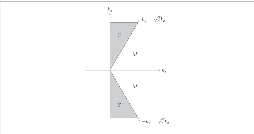
Figure1shows the distribution ofj_kin 2D wavenumber space. The dividing line is∣ ∣ky =  3kx,jkis

equal to zero in the shaded region(∣ ∣ky > 3kx)which is the zonal region with zonal(Z)modes andjkis equal

to one outside this region(∣ ∣ky < 3kx)where the modes are meridional(M)modes. The dividing line is very

important in the proposition that follows because of the structure of the manifold for the large-scale limit—for example the zonostrophy invariant is singular there. As can be seen from our proof of the proposition in appendixA, the dividing line plays an important role in showing certain triads are prohibited.

4.2. Prohibited triads

In order for the semi-action(4.8)to be conserved it must satisfy the resonance condition(3.6). So we have

= +

1 1 0for triads of typeM«M+Zand0= +0 0forZ«Z+Z. In other words, an excitation that is in aM-mode can be transferred to aM- and aZ-mode but not to twoM-modes(1¹ +1 1)or twoZ-modes

¹ +

(1 0 0)otherwise(3.6)would not be satisfied. On the other hand, an excitation that is in aZ-mode can only move to otherZ-modes and not toM-modes. This behaviour follows from the conservation of semi-action, but we would like to prove the following proposition directly.

Proposition 1.LetM≔ {k:∣ ∣ky < 3kx}be the set of meridional modes andZ≔ {k:∣ ∣ky > 3kx}be the set of zonal modes of the system with frequencywk=k kx 2. Then the following triad processes are prohibited:

(1)M«M+M,

(2)M«Z+Z,

(3)Z«M+Z,

(4)Z«M+M.

Depending on whether we are considering the kinetic or discrete regime, either one or several of the following triad processes may be realised,M«M+Zand/orZ«Z+Z.

This proposition is proven in appendixA. Note that part(4)of the proposition trivially follows from the wavenumber condition alone—it is included here solely for completeness.

4.3. Cascade directions

It was shown in Balket al(1991)for drift/Rossby WT in the case of zonally dominated turbulence,∣ ∣ky ∣ ∣kx,

and in the case of large-scale turbulence,rk1, that the presence of an additional quadratic invariant

(zonostrophy)allows us to predict the directions offluxes in thek-space of the three quadratic invariants. This is similar to the famous Fjørtoft’s argument for 2D hydrodynamic turbulence where the presence of enstrophy is shown to forbid energy toflow to small scales, and the presence of energy—to forbid enstrophyflow to large scales(Fjørtoft1953). In Nazarenko and Quinn(2009)this argument was extended to small-scale drift/Rossby turbulence,rk1. Cascade boundaries were found for the energy, enstrophy and zonostrophy: it was predicted that each of the invariants was forced by the other two to cascade into its own anisotropic sector of

k-space. A numerical study of the CHM equation was carried out which confirmed this prediction. The most straightforward application of Fjørtoft’s argument can be done to strictly positive quadratic invariants. This boils down to saying that an invariant is not allowed to dissipate in parts of thek-space where its spectral density is much less than the spectral density of at least one other invariant—otherwise the latter invariant would have to be dissipated much faster than it is produced at the forcing scales, which is impossible. This splits the entirek-space into non-intersecting sectors to which the considered invariants are allowed to cascade. Under some circumstances Fjørtoft’s argument can be extended to invariants whose density may change sign, provided that such invariants remain sign-definite in their own cascade sector of thek-space.

Below, we will return to Fjørtoft’s argument for the large-scale drift/Rossby turbulence, and revise the results of the Balket al(1991)paper by taking into account yet another quadratic invariant—the semi-actionΦ. We will modify Fjørtoft’s argument(usually formulated for a stationary forced and dissipated system)adopting it to evolving turbulence in a non-dissipative system. This is because our subsequent numerical simulations will be precisely in such an evolving non-dissipative set-up. The picture is qualitatively different depending on which sector the initial spectrum is in—zonal or meridional. Therefore, we will consider these two cases separately.

4.3.1. Initial spectrum in the zonal sector

First, let us put the initial spectrum(att=0)in the zonal sector near a wavenumberk0=(k0x,k0y)ÎZ(i.e. >

k0y k0x 3). Since the semi-action density is zero in theZ-modes, no turbulence is allowed to leave this

sector, as this would mean that initially zero semi-actionΦwould becomefinite, contradicting its conservation.

(Recall that there is no resonance triads of typeZ+Z«M.)But the zonostophyϒin the large-scale limit(4.6)

is positive in theZ-modes.

Therefore,ϒcan be used in Fjørtoft’s argument along with the other two positive invariants,EandΩ(Φwill not be involved in this argument as it is zero in this case). Namely, let us supposead absurdumthat att>0a significant proportion of a particular invariant(of the order of its total value)has moved into the vicinity of a scalekwhere the density of this invariant is much less than the density of at least one of the other two invariants. But then the amount of such an invariant with the dominant density would have at the scales aroundkan amount which is greatly exceeding its total initial value. This would contradict conservation of this invariant and, is therefore, impossible.

Thus, the entirek-space could be divided into three sectors to which respective invariants are allowed to

flow. The boundaries of these sectors are‘soft’in a sense that the invariants are allowed to cross into each other’s sector but not too deeply. These boundaries can be found by equating the ratios of densities for each pair of invariants to their initial value, i.e.:

• W¡:

( ) ( )

k k

2 2

y x

y x

0

0

• E¡:_⎣⎢⎡

( )

( )

k k 2

2 2

02

y x

y x

0

0

The resulting cascade picture is summarised infigure2. It can been seen that the energy cascades to largek,

the enstrophy to smallk,both becoming progressively more zonal, and the zonostrophyflows towards theZ/M

boundaryky= 3kx(without crossing it).

4.3.2. Initial spectrum in the meridional sector

Let us now put the initial spectrum(att=0)in the meridional sectorMnear a wavenumber

=(k k )ÎM

k0 0x, 0y (i.e.k0y k0x< 3). It is clear that invariantΦmust remain inMbecause its density is zero

outside of this sector. However,EandΩare free toflow fromMtoZ. In this case zononstophyϒis not sign-definite and, therefore, cannot restrict thefluxes of the other quadratic invariants. On the other hand, semi-actionΦis now non-zero and positive and, therefore, must be used in Fjørtoft’s argument along with the other two positive invariants,EandΩ.

In this case, the cascade boundaries obtained by the pairwise equating of the invariant densities are:

• EW:k2=k , 02

• EF:k kx 2=k k0x 02, kÎM, • WF:kx=k0x, kÎM.

TheEWboundary separates theE- and theΩ-cascades: as before it means thatEcannot be transferred to

kk0andΩ—tokk0. Further, since theEFand theWFboundaries are only inM, we havek 2kxk.

So, because the boundaries are‘soft’, we can takekx~k, andfind that all three boundaries,EW,EFandWF,

approximately coincide inM. This means thatΦcannotflow to largek, and, assuming that it should move far from the initial scalek0, it must move to modes with smallk(while remaining inM). On the other hand,Ω

cannot be transferred to neither large nor small wave vectors inM. The only remaining choice forΩis toflow to small wave vectors inZ. The latter choice does not contradict conservation ofΦbecause its density is zero inZ. A summary for the allowed cascade directions for this case is given infigure3.

5. Numerics

In order to test numerically our theoretical predictions, a pseudo-spectral code using a third-order Runge–Kutta time integration algorithm, originally used for the small-scale case in Nazarenko and Quinn(2009), has been used after adapting it to the large-scale limit—(3.1)with frequencywk=k kx 2and interaction coefficient(4.4).

Figure 2.Cascade directions when the initial spectrum is in theZsector. Dashed line is theZ/Mboundary. Bold solid lines are the W

Similarly to the original set-up, we use initial condition:

y = = +f +

-ˆ ∣ ( )

∣ ∣

*

⎜ ⎟

⎛

⎝ ⎞⎠

Ae image, 5.1

t k 0 i k k k k 02 2

—a Gaussian spot centred atk0with widthk*and its mirror image with respect to thekx-axis. Phasesfkare are

chosen to be random using a random number generator and independent andAis a constant controlling the level of nonlinearity. For simplicity we take the size of the periodic box asL=2p. We will consider cases when the initial spectrum is in the zonal sectorZand in the meridional sectorM(the Gaussian is suitably truncated to ensure that the initial condition is fully concentrated in one sector only), and cases with both weak and strong nonlinearity. Our theoretical set up is such that interactions are weak. However, more typically nonlinearity is not always weak in all of thek-space and may become strong in some isolated parts of it. Therefore numerics are important to check if our prediction holds when we do not have a purely weakly nonlinear system.

We follow the motion of the invariants in thek-space by tracking the paths followed by their centroids defined as a meankweighted on the density of the respective invariant, i.e.:

ò

ò

ò

ò

( ) ∣ ˆ ∣

( ) ∣ ˆ ∣

( ) ∣ ˆ ∣

( ) ∣ ˆ ∣ ( )

∣ ∣ t E k t t Z k k k t k

k k k

k k k

k k k

k k k

1

d ,

1

d ,

1

3 d ,

1

d . 5.2

E k k Z k x y x

k k k _x

k k k k 0 2 2 0 2 0 2 2 2 2 0, 3 2 x x x

x y x

Here we took into account(4.3)according to whichnk =∣ ˆ ∣yk2 kx(remember thatL=2p). The centroids

mark the positionkaround which most of the respective invariant is concentrated in thek-space at timet.

5.1. Initial spectrum in the zonal sector

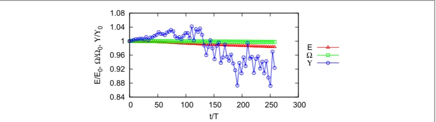
Let us put the initial spectrum in the zonal sector and start with weak nonlinearity. We take the following parameters:k0=(20, 65 ,) k_*=8,b =10, A= ´5 10-5and a resolution of 5122. Figure4shows the

evolution of the total energy, enstrophy and zonostrophy. Here, timetis normalised to the period of the mode

k0, i.e.T=2p w( )k0. It can be seen that the energy, enstrophy and zonostrophy are conserved to within 1.7%, 0.3%and 18% respectively. Conservation of the energy and enstrophy is a good test of the numerical

method because these are exact invariants of the underlying equations in the periodic box for any level of nonlinearity. Slightly poorer conservation of the energy is expected since this quantity has a higher contribution from the largek-modes which evolve faster and, therefore, are more sensitive to the error due to afinite time step. On the other hand, zonostrophy is an approximate invariant whose conservation depends on the nonlinearity level.

For the resolution we initially used 2562and found that the results are very similar suggesting that there is not much sensitivity to resolution, except for better conservation of the energy and the potential enstrophy at512 .2

Although it may seem that this resolution is modest for theses days, to simulate weakly nonlinear systems it is not as they take a long time, evolving very slowly.

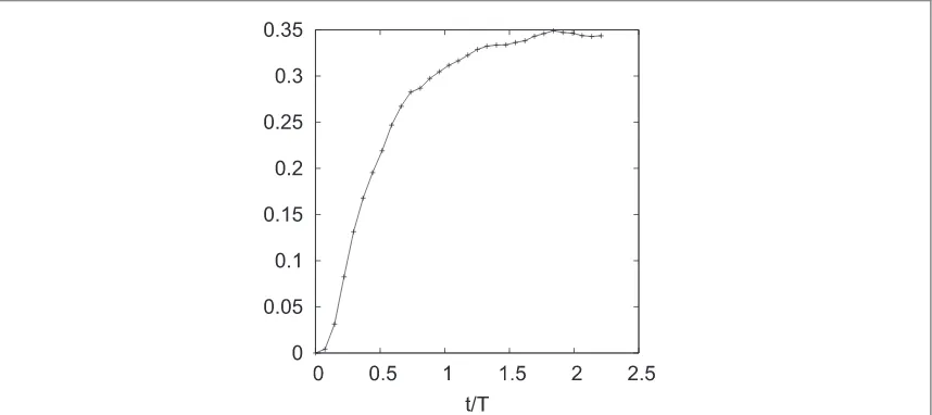
Figure5shows the ratio of the semi-action to the total action in the system. This ratio is chosen as an indicator of the semi-action conservation, obviously, considering the relative change of this invariant based on its initial value would be meaningless as the latter is zero. From this plot we see that the prediction that weak turbulence initially contained if the zonal sector will remain there indefinitely holds with very high accuracy. Indeed, less than0.6%of action escapes into the meridional sector.

Figure6shows paths of the centroids of the energy, enstrophy and zonostrophy normalised to the initial positionk0. One can see that the invariants move into the sectors predicted in section4.3.1.

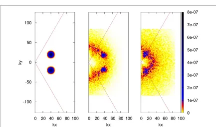
Theψ-spectrum in 2Dk-space is shown infigure7. As previously seen infigure5, the spectrum remains in the zonal sector. The spectrum evolves towards the origin with zonalflow forming at two distinct places— stronger one in a lowkregion and a weaker one with highkʼs. The latter forms near the zonal scalek~(0,k0y)

in agreement with a theoretical prediction of Nazarenko(1991).

In our next run the amplitude was increased toA= ´1 10-3_{so as to make the system strongly nonlinear.}

Figure8shows evolution of the total energy and enstrophy. Like before, we see that the enstrophy is conserved considerably better than the energy. On the other hand, zonostrophy is not conserved at all and, therefore, not shown(its variations exceed 300% of its initial value). Figure9shows the ratio of the semi-action to the total action in the system. We can see that the semi-action is not conserved, and turbulence is no longer contained in the zonal sector.

Centroid paths of the energy and enstrophy are shown infigure10. As the zonostropy is not conserved, it is not expected to restrict the energy and enstrophyfluxes, and, therefore, we are not showing its centroid. On the other hand, the energy and enstrophy still restrict transfer directions of each other in accordance with the predictions of Fjørtoft’s argument(which reduces to the standard argument as in 2D turbulence in this case).

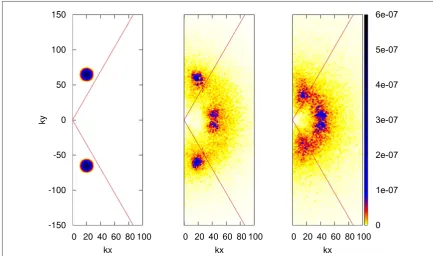
Drastic differences with the weakly nonlinear system are particularly evident on the 2D spectra shown in

figure11. Now that nonlinearity is strong and three-wave resonances are no longer dominant, proposition1no

Figure 4.Evolution of the energy, enstrophy and zonostrophy when the initial spectrum is in the zonal sector and nonlinearity is weak.

Figure 5.Plot showing the ratio of actionnkin the meridional sector(semi-action)to that in the whole ofk-space when the initial

Figure 6.Centroid paths of the energy, enstrophy and zonostrophy when the initial spectrum is in the zonal sector and nonlinearity is weak.

Figure 7.Three frames of theψ-spectrum in 2Dk-space when the initial spectrum is in the zonal sector and nonlinearity is weak.

longer confines turbulence to the zonal sector only. It can be seen that the spectrum moves into the meridional sector, initially exciting near-meridional modes with wavenumbers close to the sum of the dominant

wavenumbers in the initial Gaussian and its image. Subsequent evolution is characterised by isotropisation of the spectra.

5.2. Initial spectrum in the meridional sector

Let us now put the initial spectrum in the meridional sector. Namely, we take the initial spectrum as in(5.1)with

=( )ÎM

k0 40, 20 and with a width ofk_*=8.In our next run the initial amplitude was chosen as

= ´

-A 1.875 10 4_{so as to make the run weakly nonlinear. The resolution was 256}2

.

Figure12shows the evolution of the energy, enstrophy, zonostrophy and semi-action. The energy, enstrophy and semi-action are well conserved to within3%, 1%and 7% respectively. The zonostrophy is also conserved initially, but its conservation breaks down rather abruptly in the second half the runtime. This probably happens when the turbulent spectrum reaches the zonal/meridional boundary at which the zonostrophy density(4.6)becomes singular, which has a detrimental effect for the conservation conditions.

Figure13shows the cascade directions of energyE,enstrophyΩand semi-actionΦplotted in terms of the centroid paths. It can be seen that each invariant cascades in the direction predicted in section4.3.2. However,Ω has not reached its designated low-kcorner of the zonal sector. Interestingly, to get to this sector the centroid of

Ωhas to cross the region of low-kmeridional scales which is forbidden in a sense that no significant amount ofΩ can be present in it at any time. But this means that the transfer occurs nonlocally—passing directly from the initial to the destination scales. At intermediate times this would correspond to two spots in the 2Dk-space with

Figure 9.Plot showing the ratio of actionnkin the meridional sector to that in the whole ofk-space when the initial spectrum is in the

zonal sector and nonlinearity is strong.

Figure 11.Three frames of theψ-spectrum in 2Dk-space when the initial spectrum is in the zonal sector and nonlinearity is strong.

Figure 12.Evolution of the energy, enstrophy, zonostrophy and semi-action when the initial spectrum is in the meridional sector and nonlinearity is weak.

significant concentration ofΩ, both of which would contribute to the centroid ofΩplacing it somewhere in between, i.e. in meridional scales.

Figure14shows three frames of theψ-spectrum in 2Dk-space at the start, during and at the end of the run. As described in the previous paragraph, we see signs of nonlocal excitation of turbulence bypassing intermediate regions of thek-space. The scales excited are actually on theZ/Mboundary, which is allowed by Fjørtoft’s argument(recall that the cascade boundaries are‘soft’). Evolution of initially meridional spectrum toward the

Z/Mboundary was previously reported by Saito and Ishioka(2013).

To see what happens when nonlinearity is increased, we perform a run with initial amplitude

= ´

-A 1 10 3_{, and with the rest of the parameters as before. Figures15–17show the evolution of the invariants,}

cascade directions and theψ-spectrum respectively. The zonostrophy line has been removed from the evolution plot as it quickly looses conservation. The energy, enstrophy and semi-action are conserved to within3.5%, 1%

and 17% respectively. A word of caution is due about the 17% conservation of the semi-action, which might not seem bad at thefirst sight. Imagine a situation when thefinal spectrum is fully isotropic: the waveaction loss into the zonal sector would only be 30% in this case.

Secondly, one has to be cautious interpreting the cascade directions infigure16which seem to be quite similar to the weakly nonlinear case. In fact, the spectrum evolution seen infigure17is drastically different than before: the spectrum evolution is more gradual/local and with a strong tendency to isotropisation, which is expected for strongly nonlinear systems. It is this isotropisation that explains the motion of the centroids in

figure16(along with the usual tendency forEandΩto go to the large and smallkʼs respectively).

Figure 14.Three frames of theψ-spectrum in 2Dk-space when the initial spectrum is in the meridional sector and nonlinearity is weak.

6. Finite-

ρ

effects

So far we have studied the large-scale limit(r0)for which we proved proposition1about the forbidden triads. However, we would also like to see what happens whenρis small butfinite. It turns out that some

+ «

Z Z Mtriads which are forbidden forr0start to appear. They contain wave vectors close to theZ/M

boundary for which the deviation ofk ky xfrom 3shrinks asr0.In other words, asρincreases, the angle

containing forbidden triads around theZ/Mboundary also increases. See below. Fixingk=(cos , sinq q)in the resonant conditions(2.12), infigure18we plotk ky x- 3for resonantZ+Z«Mtriads as a function ofr2

for three different values ofθ. We see that the closerθis to the boundary, the bigger the angle containing

+ «

Z Z Mtriads.

We have further found that the triadsM+M«MandM+Z«Z(and obviouslyM+M«Z)

forbidden inr0limit, continue to be absent forfinite but smallρ.

To check if our numerical results obtained for the large-scale limit are robust whenρis increased, we performed simulations of the full CHM equation(2.1)withF=100 000.For our typical modes this

corresponds torkin the range from 0.1 to 0.4, which is not so small for formal validity of therk0limit. We

Figure 16.Centroid paths of the energy, enstrophy and semi-action when the initial spectrum is in the meridional sector and nonlinearity is strong.

use the full CHM equation(2.4)in Fourier space with frequency(2.5)and interaction coefficient(2.6). Again, we considered a set of four cases when the initial spectrum was in the zonal and meridional sectors, and also when the nonlinearity was both weak and strong. The results of this study are reported in appendixB: they reproduce all of the qualitative features of the results obtained for the large-scale limit. This demonstrates that, at least qualitatively, the mechanisms discovered for ther0limit remain at work for large-scale turbulence withrk0.4.

7. Conclusion

For the large-scale limit of the CHM equation, a new quadratic invariant has recently been discovered in Saito and Ishioka(2013)for weakly nonlinear systems; it is called the semi-actionΦin the present paper—see(4.7)

and(4.8). Prompted by the fact of its conservation, we have proposed and proven that the following resonant triads are prohibited,M«M+M M, «Z+Z Z, «M+ZandZ«M+M, whereZandMare the zonal and meridional sets of modes defined in proposition 1. This proposition has a drastic consequence for the weakly nonlinear dynamics of the large-scale CHM systems: spectrum initially fully concentrated in the zonal sectorZcannot ever leave this sector(noM-modes can be excited).

Another additional quadratic invariant of the large-scale CHM equation, known since 1990(Balket al1990, Nazarenko1990and Balket al1991)—is zonostropyϒdefined in(3.7)and(4.6). In these papers it was used in a generalised Fjørtoft’s argument resulting in a triple cascade picture of anisotropic drift/Rossby turbulence. In the present paper, we have used the newly discovered semi-action invariant to revise Fjørtoft’s argument. The latter is now presented in a modified version for evolving non-dissipative systems assuming that the quadratic invariants will eventually move to scales which are greatly separated from the initial scalek0. If the initial

spectrum is inZthen it remains inZ, but the invariants are transferred among the zonal scales. Namely, the energy cascades to large zonalkʼs, the enstrophy—to small zonalkʼs, and the zonostrophy—towards the the

Z/Mboundary,ky= 3kx. If the initial spectrum is inMthen energy cascades towards largekʼs, enstrophy—

to small zonalkʼs, and semi-action—to small meridionalkʼs(by definition, the latter cannot leaveM). We have tested and confirmed our theoretical predictions numerically. In particular, we have confirmed conservation of the semi-action and zonostrophy invariant. We also confirmed that when nonlinearity is weak

(three-wave interactions dominate)turbulence which is initially inZremains inZwith remarkable a0.6%

accuracy. In this case, it is redistributed within the zonal sector with the energy, enstrophy and zonostrophy moving in the 2Dk-space as predicted by Fjørtoft’s argument. The 2D spectrum develops two distinct components: the main spot that spreads to zonal scales with smallerkʼs and a smaller spot forming with large-k

zonal scales neark~(0,k0y)(formation of the latter was predicted in Nazarenko(1991)).

When nonlinearity is weak and turbulence is initially inM,the spectrum tends to move towards and concentrate near theZ/Mboundary,ky= 3kx.Such a behaviour was previously reported in Saito and Ishioka (2013). The cascade directions appear to be qualitative predictions of Fjørtoft’s argument. Notably, conservation of the zonostrophy, which holds initially, is suddenly broken down when the spectrum reaches theZ/M

boundary on which the density of this invariant is singular.

When nonlinearity is increased, as expected, for both zonal and meridional initial conditions, conservation of the semi-action and(especially)zonostropy deteriorates. In particular, initially zonal turbulence is no longer

Figure 18.The angle from theZ/Mline containing resonantZ+Z«Mtriads as a function ofr2_{forq=5p 16, 10p 31and} p

contained in the zonal sector. Turbulence evolution shows tendency to isotropisation, as expected for strongly nonlinear CHM, because the linear term is the only source of anisotropy in this model. In general, the system evolves similar to the classical 2D turbulence, but with reversal of roles of the energy and the enstrophy—they cascade to the small and large scales respectively in our case.

We have also studied sensitivity of our results to increasing values ofρ, so that formally the CHM system is not in the large-scale limit. We showed that even for small values ofρ, some resonant triads of typeM«Z+Z

(but not the other types forbidden in the large-scale limit)exist. They appear with wavenumbers close to the

Z/Mboundary, and the sector in which they exist grows asρincreases. Thus, forfinite but smallρ,‘leakage’ between theZandMsectors occurs primarily near theZ/Mboundary only. Using direct numerical simulations of the CHM equation, we have found that most of the qualitative and even quantitative features of the large-scale limit survive for our numerical set-ups up to valuesrk0.4.

Acknowledgments

Katie Louise Harper gratefully acknowledges EPSRC DTA funding of her PhD studies.

Appendix A. Proof of proposition 1

Letk=(p q, ),p>0andw=p p( 2+q2)._{Let us begin by writing out the frequency resonance condition,}

w =w1+w2, in which we substitute the wavenumber resonance condition,k=k1+k2:

+ = + + - - +

-( ) ( ) ( )(( ) ( ) ) ( )

p p2 q2 p p q p p p p q q . A.1

1 1 2

1 2

1 12 12

Solving the quadratic equation, we have forq1:

= 

 ( )

q p q

p p 1 , A.2 D 1 2 4 with: = + + ( ) D

p q p p p p pq

4 2 3 . A.3

2 2 2

1 2 1 2

Takingq>0we can see thatq₁₊>0andq_1-<0.Usingq_2= -q q_1gives:

=

 ( )

q p q

p p

D

1

4 , A.4

2

1 _

whereq₂₊<0andq_2->0.

We mustfirst prove thatq_1 p₁andq_2 p₂are monotonic functions in the interval0<p_1,2<p,i.e. they have no local extrema in this range. From(A.2)and(A.3)we have:

= -  - + + - (( ) ( )) ( ) q p q p q

p pp p p p p q p p p p

1

3 . A.5

1

1 1 1 1

2

1 2 2 2 1 1 1 2

Differentiating with respect top1

¶ ¶ = -- + + - - + -- + + - (( ) ( )) ( ) (( ) ( )) ( ) ⎛ ⎝ ⎜ ⎞ ⎠ ⎟ p q p q p

p p p p q p p p p

pp

q p p p p p

pp p p p p q p p p p

3

2 3 6

2 3 A.6

1 1 1 1 2 1 2

1 2 2 2 1 1 1 2

1 2

2

1 3 2 1

1 1 2

1 2 2 2 1 1 1 2



and setting the result to zero, we get:

- - - = ( )

⎜ ⎟

⎛

⎝ ⎞⎠

p q 9p q p q

4 3 2

1

4 0. A.7

1

2 4 4 2 2 4

¶ - + -+ - + -( ) ( ( ) ) ( ) ⎝ ⎜ ⎠ ⎟

p p p pp

q p p p p p

pp q p p pp p p p p

2 3 6

2 3 3 . A.9

2 2 2

2

2 2

2

2 3 2 2

2 2 2

2 2

2 3 2 2

2 2 1 2 

Rearranging and setting the result to zero, we have:

- + = ( ) ⎛ ⎝ ⎜ ⎞ ⎠ ⎟

p q p

q p 3 4 9 4 3

2 0, A.10

2

2 2 4

2 2

from which it can be seen thatp₂ =0,so again there are no extrema in the range0<p₂ <p,which is the same as0<p₁<p.

Thus, we have proven thatq_1 p₁andq_2 p₂are monotonic functions in the interval0<p_1,2 <p. Now, we need tofind out whetherq_1 p₁andq_2 p₂are monotonically increasing or monotonically decreasing functions ofp₁.To do this we must compare their values atp₁0andp₁p.

(i) Let usfirst consider the limitp₁0 (p₂p). From(A.5)we have:

 -  + - -  + - ( ) ( ) ( ) ⎛ ⎝ ⎜ ⎞ ⎠ ⎟ ⎡ ⎣ ⎢ ⎤ ⎦ ⎥ q p q p q p q p p q pq p q p q p q p p q pq p 1 3 1 3

2 . A.11

1

1 1 1

2 2 2 1 1 2 1 1 2 2 2 1

Therefore, we can see that:

  +¥ + ( ) q p q p 2 A.12 1 1 1

(sincep₁ 0)and:

 - -- _{( )} q p q p p q 2 3

2 . A.13

1 1 Respectively   ( ) q p q

p. A.14

2

2 

(ii) Now, let us consider the limitp₁p (p₂0). From(A.8), ignoringp₂2terms, we have:

  + - ( ) ( ) ⎡ ⎣ ⎢ ⎤ ⎦ ⎥ q p p q p q p p q pq p 1 3

2 , A.15

 - -+ ( ) q p q p p q 2 3

2 . A.18

2

2

Therefore we can see thatq_1 p₁are monotonously decreasing functions andq_2 p₂are monotonously increasing functions ofp1.

Let us denotex=q p>0.For the right-hand sides of(A.13)and(A.18)we have:

= -

-( ) ( )

f x x

x

1 2

3

2 . A.19

This function has a single maximum atx= 3at which f= - 3. Hence, the maximum value ofq_1- p₁and +

q₂ p₂is always- 3(the equal sign is realised whenkis on theZ/Mboundary,x= 3.

Let us consider the caseq>p 3 ,i.e.kÎZ. A graph summarising ourfindings for this case is presented in

figureA1. It can be seen that:

> > + _ - _{ ( )} q p q p q p q p

3 , 3 . A.20

1

1

2

2

Together with the relations:

< - <

-- + ( )   q p f q p f

3 , 3 , A.21

1

1

2

2

these inequalities mean thatk1ÎZandk2ÎZ. Thus, we have proven parts(3)and(4)of proposition1.

Let us consider now the caseq<p 3 ,i.e.kÎM. A graph summarising ourfindings for this case is presented infigureA2. We can see that all curves change between the setsM«Zat some pointsp1within the

range0<p₁<p.We need to prove that these points coincide forq₁₊ p₁andq₂₊ p₂(we will call itp₊*)as well as forq_1- p₁andq_2- p₂(we will call itp_-*).

For this we willfirst rewrite the intersection condition:

= = +

+ ( )

q p p q

p p

D

3 1

4 , A.22

1 1 2

as:

- = + +

( 3p p₁ p q₂ )2 p q 3p p p p pq . (A.23) 2

2 2 2

1 2 1 2

Since at the intersectionp₁¹0, we get:

= ₊* = + = - ( )

p p p q p p q

2 2 3 or 2 2 3. A.24

1 2

From this we can see that:

< + < « < ( )

p p if p q p q p

3 2 3 , A.25

1

i.e. the intersection exists whenkÎM, as it is the considered case.

Now consider intersection:

= - =

-+ ( )

q p p q

p p

D

3 1

4 , A.26

2 2

1

leading to:

+ = + +

( 3p p₂ p q₁ )2 p q 3p p p p pq (A.27)

22 2 2 1 2 1 2

and:

= - ( )

p p q

2 2 3. A.28

2

Thus, we have proven that this intersection point is the same as(A.24), as required.

Similarly, one proves that intersectionsq_1- p₁= 3andq_2- p₂ = 3are achieved at the same point

= _-*

p₁ p given by:

=

--* ( )

p p q

2 2 3. A.29

But this means thatk1andk2cannot be simultaneously inM, nor they can be simultaneously inZ. So we have

proven parts(1)and(2)of the proposition1.

Appendix B. Numerical results for the cases when

ρ

is small but

fi

nite

Let us consider a case when the initial spectrum is in the zonal sector. For the weak nonlinearity run, we chose a resolution of512 ,2 k =(20, 65 ,) k_*=8,b=10

0 andA =7.5´10-9. FiguresB1–B3show the

conservation and cascade directions of the energy, enstrophy and zonostrophy and theψ-spectrum respectively. For the strongly nonlinear run we increased the amplitude toA= ´1 10-7_{. The numerical plots are}

presented infiguresB4–B6.

For the weakly nonlinear run with a meridional initial condition the resolution was

b

=( ) k_*= =

k

256 ,2 40, 20 , 8, 10

0 andA =1.875´10-8. FiguresB7–B9show the conservation of the

energy, enstrophy, zonostrophy and action, the cascade directions of the energy, enstrophy and semi-action and the 2Dψ-spectrum respectively.

For the strongly nonlinear runfiguresB10–B12, we increased the amplitude toA = ´1 10-6_{and kept the}

remaining parameters the same.

We see a remarkable agreement of the above plots obtained for both weak and strong initial conditions in both zonal and meridional sectors with the respective plots reported in the main text of the large-scale limit simulations.

Figure B1.Evolution of the energy, enstrophy and zonostrophy when the initial spectrum is in the zonal sector, nonlinearity is weak andρis small butfinite.

Figure B2.Centroid paths of the energy, enstrophy and zonostrophy when the initial spectrum is in the zonal sector, nonlinearity is weak and_ρis small but_finite.

Figure B4.Evolution of the energy and enstrophy when the initial spectrum is in the zonal sector, nonlinearity is strong andρis small butfinite.

Figure B5.Centroid paths of the energy and enstrophy when the initial spectrum is in the zonal sector, nonlinearity is strong andρis small butfinite.

Figure B7.Evolution of the energy, enstrophy, zonostrophy and semi-action when the initial spectrum is in the meridional sector, nonlinearity is weak andρis small butfinite.

Figure B8.Centroid paths of the energy, enstrophy and semi-action when the initial spectrum is in the meridional sector, nonlinearity is weak andρis small butfinite.

Figure B10.Evolution of the energy, enstrophy and semi-action when the initial spectrum is in the meridional sector, nonlinearity is strong andρis small butfinite.

Figure B11.Centroid paths of the energy, enstrophy and semi-action when the initial spectrum is in the meridional sector, nonlinearity is strong and_ρis small but_finite.

References

Balk A M 1991 A new invariant for Rossby wave systemsPhys. Lett.A15520–4

Balk A M, Nazarenko S V and Zakharov V E 1990 On the structure of the Rossby/drift turbulence and zonalflowsProc. Int. Symp. on Generation of Large-scale Structures in Continuous Media (Moscow, 11–20 June)ed G Moiseey and V V Moshev(Moscow: Space Research Institute)pp 34–5

Balk A M, Nazarenko S V and Zakharov V E 1991 A new invariant for drift turbulencePhys. Lett.A152276–80

Charney J G 1948 On the scale of atmospheric motionsGeophys. Public173–17

Connaughton C, Nazarenko S and Quinn B 2015 Rossby and drift wave turbulence and zonalflows: the Charney–Hasegawa–Mima model and its extensionsPhys. Rep.6041_–71

Gürcan Ö D and Diamond P H 2015 Zonal_flows and pattern formationJ. Phys. A: Math. Theor.48293001

Diamond P H, Itoh S I, Itoh K and Hahm T S 2005 Zonalflows in plasma—a reviewPlasma Phys. Control. Fusion4735–161

Dorland W, Hammett G W, Chen L, Park W, Cowley S C, Hamaguchi S and Horton W 1990Bull. Am. Phys. Soc.352005

Fjørtoft R 1953 On the changes in the spectral distribution of kinetic energy for two-dimensional non-divergentflowTellus5225–30

Glazman R E and Weichman P B 2005 Meridional component of oceanic Rossby wave propagationDyn. Atmos. Oceans38173

Harper K L, Bustamante M D and Nazarenko S V 2013 Quadratic invariants for discrete clusters of weakly interacting wavesJ. Phys. A: Math. Theor.46245501

Hasegawa A and Mima K 1978 Pseudo-two-dimensional turbulence in magnetised nonuniform plasmaPhys. Fluids2187–92

Horton W and Ichikawa Y H 1996Chaos and Structures in Nonlinear Plasmas(Singapore: World Scientific)

L’vov V S and Nazarenko S V 2010 Discrete and mesoscopic regimes offinite-size wave turbulencePhys. Rev.E82056322

Nazarenko S 2011Wave Turbulence(Lecture notes in Physicsvol 825) (Berlin: Springer)

Nazarenko S and Quinn B 2009 Triple cascade behaviour in QG and drift turbulence and the generation of zonal jetsPhys. Rev. Lett.108501 Nazarenko S V 1990Physical Realisability of Anisotropic Spectra of Wave Turbulence and Structure of the Rossby/Drift Turbulence(Moscow:

Landau Institute for Theoretical Physics)

Nazarenko S V 1991 On the nonlocal interaction with zonalflows in turbulence of drift and Rossby wavesSov. Phys.—JETP53604–7 Petviashvili V and Pokhotelov O 1992Solitary Waves in Plasmas and in the Atmosphere(London: Taylor and Francis)

Saito I and Ishioka K 2013 Angular distribution of energy spectrum in two-dimensionalβ-plane turbulence in the long-wave limitPhys. Fluids25076602

Smolyakov A I, Diamond P H and Shevchenko V I 2000 Zonal_flow generation by parametric instability in magnetized plasmas and geostrophicfluidsPhys. Plasmas71349–51

Zakharov V E and Schulman E I 1980 Degenerative dispersion laws, motion invariants and kinetic equationsPhysicaD1192–202