Asynchronous coupling of hybrid models for efficient simulation of multiscale systems

http://wrap.warwick.ac.uk

Lockerby, Duncan A., Patronis, Alexander, Borg, Matthew K. and Reese, Jason M..

(2014) Asynchronous coupling of hybrid models for efficient simulation of multiscale

systems. Journal of Computational Physics, 284 . pp. 261-272.

Permanent WRAP url:

http://wrap.warwick.ac.uk/77101

Copyright and reuse:

The Warwick Research Archive Portal (WRAP) makes this work of researchers of the

University of Warwick available open access under the following conditions.

This article is made available under the Creative Commons Attribution 4.0 International

license (CC BY 4.0) and may be reused according to the conditions of the license. For

more details see:

http://creativecommons.org/licenses/by/4.0/

A note on versions:

The version presented in WRAP is the published version, or, version of record, and may

be cited as it appears here.

Contents lists available atScienceDirect

Journal

of

Computational

Physics

www.elsevier.com/locate/jcp

Asynchronous

coupling

of

hybrid

models

for

efficient

simulation

of

multiscale

systems

Duncan A. Lockerby

a

,

∗

,

Alexander Patronis

a

,

Matthew K. Borg

b

,

Jason M. Reese

c

a_{SchoolofEngineering,UniversityofWarwick,CoventryCV47AL,UK}

b_{DepartmentofMechanical&AerospaceEngineering,UniversityofStrathclyde,GlasgowG11XJ,UK} c_{SchoolofEngineering,UniversityofEdinburgh,EdinburghEH93JL,UK}

a

r

t

i

c

l

e

i

n

f

o

a

b

s

t

r

a

c

t

Articlehistory:

Received6August2014

Receivedinrevisedform16December2014 Accepted20December2014

Availableonline24December2014

Keywords:

Multiscalesimulations Unsteadymicro/nanoflows Hybridmethods Scaleseparation Rarefiedgasdynamics

Wepresent anewcouplingapproachforthetimeadvancementofmulti-physicsmodels of multiscale systems. This extendsthe method ofE et al. (2009) [5] to dealwith an arbitrary number of models. Coupling is performed asynchronously, with each model being assigned its own timestep size.This enables accurate longtimescale predictions to bemadeatthe computational costof theshort timescale simulation.We proposea methodforselectingappropriatetimestepsizesbasedonthedegree ofscaleseparation thatexists betweenmodels.Anumber ofexampleapplicationsare used fortestingand benchmarking, including a comparison with experimental data of a thermally driven rarefiedgasflowinamicrocapillary.Themultiscalesimulationresultsareinveryclose agreementwiththeexperimentaldata,butareproducedalmost50,000timesfasterthan fromaconventionally-coupledsimulation.

©2014TheAuthors.PublishedbyElsevierInc.ThisisanopenaccessarticleundertheCC BYlicense(http://creativecommons.org/licenses/by/4.0/).

1. Introduction

Amulti-physicsdescription ofa multiscalesystemisoftenreferredto asa ‘hybrid’model.Influid dynamics,a typical hybridcombines amolecular treatment(a‘micro’model)witha continuum-fluidone(a‘macro’ model),withtheaimof obtaining theaccuracy oftheformer withtheefficiencyofthe latter[1–4].Themicro andmacromodelsgenerallyhave characteristictimescalesthatareverydifferent,whichmeansthattime-accuratesimulationscanbeextremelychallenging: thesizeofthetimesteprequiredtomakethemicromodelstableandaccurateissosmallthatsimulationsoversignificant macro-scaletime periodsareintractable.Ifthesystemis‘scale-separated’,aphysical(asdistinctfromnumerical) approxi-mationcanbemadethatenablesthecoupledmodelstoadvanceatdifferentrates(asynchronously)withnegligiblepenalty onmacro-scaleaccuracy.Eetal.[5]werethefirsttointroduceandimplementthisconceptinatime-steppingmethodfor coupledsystems,referredtointheclassificationofLockerbyetal.[6]asacontinuousasynchronous(CA)scheme (‘contin-uous’sincethemicroandmacromodelsadvancewithoutinterruption[5]).Inthispaperweextendthisideatomultiscale systemscomprisinganarbitrarynumberofcoupledmodels.

*

Correspondingauthor.

E-mailaddress:[email protected](D.A. Lockerby).

http://dx.doi.org/10.1016/j.jcp.2014.12.035

[image:3.561.129.423.57.215.2]

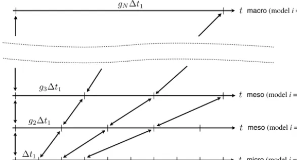
Fig. 1.The continuous asynchronous (CA) coupling scheme extended to multi-model multiscale systems.

2. Extensiontomulti-modelsystems

WeconsideranN-modeltimescale-separatedsystem,wheretheithmodelhasacharacteristictimescaleTi,andindexing isorderedsuchthat

Ti

≤

Ti+1 fori

=

1

, . . . ,

N

−

1

.

(1)

Modeli

=

1 isthemicromodelandi

=

N isthemacromodel;modelsi

=

2 toi

=

N

−

1 are‘meso’models.Thedegreeof scaleseparation Si betweenmodeli andi

+

1 is

Si

=

Ti+1

Ti

≥

Stol

,

(2)

wherethetolerance Stolrequireseachdistinctmodelofthesystemtobescaleseparatedfromeveryothertosomedegree,

for example, Stol

=

O

(

10

)

. If this condition is not met, the two models are treated as one, and coupling is performed

conventionally.

Ingeneraleachmodelcanbeconsideredtohaveitsowntimevariable(ti),andberepresentedby d Xi

dti

=

F

i

X

(

ti

)

,

(3)

where Xi are the set of variables of the ith model, and

F

i is some function of the complete system’s variables, X

=

{

X1

,

X2

,

. . . ,

XN

}

. It is important to make clearthe distinction between the characteristic timescale ofthe ith model in isolation(Ti)andthetimescaleofitsvariableswithinthecoupledsystem;theyare,potentially,completelydifferent.

Tosolvethissetofmodels,theindependenttimevariablesmustberelatedtoeachother.Ifalltimevariablesareequal (i.e.t

=

t1...N) thesystemisconventionallycoupled.However, wecan advancemodelsatdifferentrateswiththephysical modification

t1

=

t2

/

g2

= · · · =

tN

/

gN

,

(4)

where gi is therate that the ith model advances relative to the micro model. Thisapproximation provides a means to exchangefinetimescaleresolutionforlongtimescalepredictions,andtheextenttowhichitisvaliddependsonthedegree ofscaleseparationbetweenmodels,i.e.onthemagnitudeof Si.Forcoupledmodels thatarehighly scaleseparated(Si

>

Stol),thesmaller-scalemodelwillremainquasi-equilibrated tothedynamicsofthelarger-scalemodeldespitethephysical

modification, and so behave similarly to as in the unmodifiedsystem. The aim is thus to represent the scale-separated system(

>

Stol) withonethatisless,butstillsignificantly,scaleseparated(

=

Stol):thisishowacceptablevaluesofgi are determined(seebelowforthespecificprocedure).Detailedanalysesoftheerrorassociatedwiththisphysicalapproximation foratwo-modelsystemaregiveninEetal.[5]andLockerbyetal.[6].

Fig. 1 provides an illustrationofa numericalimplementationofEq. (4)usingdifferenttimestep sizes foreach model, whileexchangingvariablesasifthetimestepswereequivalent(thisisasynchronouscoupling).Thetimestepoftheithmodel is

ti

=

gi

t1

,

(5)

where

t1 isthemicromodeltimestep.

[image:4.561.151.389.56.101.2]

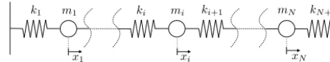
Fig. 2.A coupled mass–spring system.

1. ThephysicalapproximationofEq.(4)representsaveryscale-separatedsystembyonethatisless,butstilltoadegree, scaleseparated(i.e.hasascaleseparationofStol).Thisplacesanupperlimitontheamountatimestep ofonemodel

canbeincreasedrelativetoanother:

ti

≤

Si−1

Stol

ti−1

.

2. Thenumericalaccuracyissatisfactoryandstabilityguaranteedforeachindividualmodel:

ti

≤

ti,max

,

where

ti,maxisanestimationofthemaximumtimestepthatispermissibleforeachmodel.

Basedontheseconstraintswecansetthetimestepofeachmodelrecursively:

ti

=

min

ti,max

;

Si−1

Stol

ti−1

,

fori

=

2

, . . . ,

N

,

(6)

where

t1

=

t1,max.

Wenowconsideraseriesofexamples.TheexamplesofSections3–5areusedtoillustratetheeffectiveness,challenges, andshortcomingsofemployingthephysicalapproximationinEq.(4)andapplyingtimesteppingofEq.(6);theexampleof Section6providesademonstrationofanapplicationtohybridcontinuum-molecularmodelling.Note,thereare arangeof numericalmethodsthatcouldbeappliedtothenumerically-stiffsystemsofSections3–5,butwhichcannotbeappliedto thehybridexampleofSection6.

3. Example1:Asimplemass–springsystem

Aserialmass–spring systemwith N massesandN

+

1 springsisshowninFig. 2.Thegoverningequationsfortheith modelare d dt

vi xi

=

₁

mi

(

ki

(

xi−1

−

xi

)

+

ki+1

(

xi+1

−

xi

))

vi

,

(7)

wherexi and vi arethedisplacement andvelocity oftheithmass(mi)andki isthe ithspringconstant. Acharacteristic timescaleforeachmodelcanbeobtainedfromitsnaturalperiodinisolation:

Ti

=

2

π

mi ki

+

ki+1

.

(8)

InthisexampleN

=

5,thespringconstantsareequal,andthe

(

i

+

1

)

thmassis900

×

heavierthantheithmass,suchthat

Ti+1

=

30Ti

.

(9)

Allmodelsarethussignificantlyscale-separated.1

Thecompletesystemofequationsissolvedusingthemidpointmethod(asecond-orderRunge–Kuttascheme),butwith timestepsforeachmodelchosenaccordingtoEq.(6),with

ti,max

=

Ti

/

100.

Inthefirstcase,theinitialdisplacementsxi,t=0 arechosensuchthat,whenthemassesarereleasedfromrest,onlythe

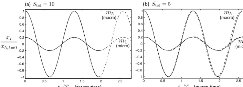
slowest eigenmode of thesystem isexcited. Fig. 3(a) showsthe response ofthe lightest (m1) and heaviest (m5) masses

governedbythemicroandmacromodels,respectively;theanalyticaleigenvaluesolution(thedashedline)is indistinguish-ablefromthe multiscalesolution.Fig. 3(b)showsthesolution using Stol

=

5, whichplaces alessconservativerestriction

onthebalancebetweenaccuracyandefficiency.ForStol=10,themodeladvances81

×

fasterthanifstandard(synchronous)

couplingwereused;forStol

=

5 itadvances1296

×

faster.

The massesare now initiallydisplaced an equal distanceand thenreleased fromrest; thisexcitesall eigenmodes, to a degree. Fig. 4 shows: (a) the response of a meso model (i

=

3) and(b) the response of the macromodel (i

=

5,the heaviestmass),forStol

=

5.Themacrodescriptionisaccurate,whileforthemesomodelonlythelowfrequencyeigenmode

isaccuratelycaptured.Thisexampleillustrates thefundamentaltrade-off requiredinmultiscaling:efficiencyinpredicting macrovariationscanbedramaticallyincreased,butattheexpenseofmicro/mesoscaleresolution.

[image:5.561.78.476.54.196.2]

Fig. 3. Normaliseddisplacement responseofthelightestand heaviestmasses(m1 andm5, respectively)toexcitationofthe slowesteigenmode.The

[image:5.561.74.475.234.376.2]

multiscaleresult(—)andananalyticaleigenvaluesolution(– –).

Fig. 4.Normaliseddisplacementresponseof(a)themedianand(b)theheaviestmasses(m3 andm5,respectively)toanequalinitialdisplacement.The

multiscaleresult(—)andananalyticaleigenvaluesolution(– –).

4. Example 2:ALotka–Volterrasystem

TheLotka–Volterraequations,invariousforms,havebeenappliedtoanextremelydiverserangeofproblems,spanning economics [7], biology [8]and chemistry [9]. Originating fromthe analysisof auto-catalytic chemical reactions [9], the equations arenowmostcommonlyusedto studythe populationdynamicsofcompetingbiologicalsystems,whichis the exampleweconsiderhere.

Thepopulationgrowthrateofaspeciesina(sequential)foodchainisasfollows:

dyi

dt

=

yi

(

−

ri

+

piyi+1

−

qiyi−1

),

(10) where yi isthepopulationsizeoftheithspecies, riistheintrinsicdeathrate(intheabsenceofanypreyorpredator), pi is thepopulationgrowthrateduetothe consumptionoflowerspeciesinthefoodchain,andqi isthedeathratedueto predationfromhigherspeciesinthefoodchain.Theintrinsicdeathrateofeachspeciesdefinesacharacteristictimescalefor that speciesmodel(ri

=

1

/

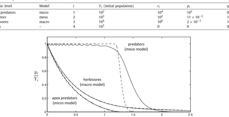
Ti),andwhichclassifiesthemodelinthemacro-to-microhierarchy;thisrateincreasesmoving upthefoodchain.Thus,theApexPredator,atthetopofthefoodchain,hasthehighestintrinsicdeathrate(intheabsence ofprey),anditspopulationsize, y1,isgovernedbythemicromodel.

Table 1 gives parameters for a food-chain example consistingof four species. For the initial population sizes Yi the ecosystem is in equilibrium, and the numbers ofeach specieswill remain constant. If, however, all plants are removed (Y4

=

0),thepopulationsoftheremainingspecieswilleventuallyreducetoextinction.Fig. 5showsthepopulationresponse

ofeachspeciesintheecosystem,aspredictedbyastandardnumericalsolution(thedashedline,usedasabenchmark)and themultiscaleapproachusingStol

=

10 (thesolidline).AsinSection3,timeintegrationisperformedusingasecond-order

Runge–Kuttamethod,withtimestepsforeach modelchosenaccordingtoEq.(6),with

ti,max

=

Ti

/

5.Forthebenchmark solution

ti

=

t1,max.

ThefirstobservationisthattheslowlyvaryingpopulationsizesoftheApexPredatorsandtheHerbivoresarepredicted veryaccuratelybythemultiscalescheme,whichis100

×

computationallyfasterthanthebenchmarksolution.Fig. 6shows the macromodelpredictionusinglessconservativetolerances ontheminimumacceptablescale separation,i.e. Stol

=

2

.

5

[image:6.561.61.501.76.302.2]

Table 1

Lotka–Volterraparametersfora4-speciesfoodchain.

Trophic level Model i Yi(initial population) ri pi qi

Apex predators micro 1 102 ₁₀4 ₁₀1 ₀

Predators meso 2 103 ₁₀2 _11×10−2 ₁₀1

Herbivores macro 3 104 ₁₀0 _2×10−5 ₁₀−3

[image:6.561.151.393.339.498.2]

Plants – 4 105 _{0 0 0}

Fig. 5.NormalisedpopulationresponsetotheinstantaneousremovalofPlants.Themultiscaleresult(—)andaconventional(benchmark)numerical solu-tion (– –).

Fig. 6.NormalisedHerbivorepopulationresponsetotheinstantaneousremovalofPlants:Stol=10 (—), Stol=5 (– –),Stol=2.5 (–·–),andabenchmark

numericalsolution(•).Note,forclarity,thebenchmarksolutionisnotplottedateverytimestep.

solutionconvergestothenumericalbenchmarkasStol isincreased;Stol

=

10 appearstoprovideaveryaccurateresultfor

themacrovariable.

However, compared to theother species, thePredators’ population decline israpid,and occursaftersome delay.The delayoccursbecause,initially,thePredators’preyandthePredators’predatorsarebothreducing–onlywhentheirpreyis significantlydiminishedisthereamajorreductioninPredatornumbers.Themultiscaleapproachdoesnotcapture,withany fidelity,theseshorterscalephenomena,andactuallyintroduceserroneousshorttimescaleoscillations.Thisagainhighlights that exploitingscale separationaffordsvery efficientpredictiononlarge timescales,butatthe expenseoffinertimescale resolution.Note,inthiscase,themicromodelpredictionisverygood,becausetheshortscaleresponseonlymanifestsitself inthemesomodel’svariable.

5. Example3:Alubricationsystem

[image:7.561.89.462.55.180.2]

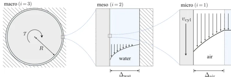
Fig. 7.Schematic of a liquid journal bearing with a lubricating air layer.

surfacetopologythat,whensubmergedinwater,combinetotrapairpocketsonthesurface.Suchcoatingshaveapplications inmarinedragreduction[10,11]andforself-cleaningsurfaces[12].Inthecontextofmultiscalemodellingtheyarerelevant becauseoftheverydifferentscalesassociatedwiththeairlayer,externalwater,andthebody/vehicle.

The bearingexampleofthissection consistsofasteelcylinder,ofradius R

=

10 cm,towhichisappliedanoscillatory torque,

T

.Thecylinderrotateswithin a fixedouter cylindercontaining water;the surfaceofthe innercylinderiscoated withan airlayerofthickness

air

=

1 μm; andtheannular thickness ofwateris

wat

=

0

.

1 mm (i.e. R

wat

air);

seeFig. 7.

Thelow-speed,unsteady,incompressibleNavier–Stokesequationsprovidemodelsfortheairlayerandthewater(i.e.the microandmesomodels,i

=

1 andi

=

2,respectively):

∂

vair

∂

t1

=

μ

air

ρ

air

∂

2vair

∂

r2

(

micro

)

(11)

and

∂

vwat

∂

t2

=

μ

wat

ρ

wat

∂

2vwat

∂

r2

(

meso

)

(12)

where r is the radial coordinate fromthe cylinder centre, v istangential velocity,

μ

is dynamic viscosity,

ρ

is density, andthesubscripts‘air’and‘wat’denotetherespectivefluids. Giventhat R

wat

air,thecurvatureofthegeometry

can beneglected.The microandmeso modelsarecoupledbytherequirementfortheshearstressandthevelocitytobe continuousattheair–waterinterface(assumingnoslip):

μ

air dvair

dr

r=rint

=

μ

wat

dvwat dr

r=rint

,

(13)

and

vair

|

r=rint

=

vwat

|

r=rint

,

(14)

wheretheradialpositionoftheair–waterinterfaceisrint

=

R

+

air.Thewateratthewalloftheoutercylinderisstationary

(i.e.thereisnoslip).

Newton’ssecondlawdeterminestheevolutionofthetangential velocityoftheinnercylindersurface (vcyl);thisisthe

macromodel(i

=

3):

∂

vcyl

∂

t3

=

R I

2

π

L R2

μ

air

∂

vair

∂

r

r=R

+

T

(

t3

)

(

macro

)

(15)

where L isthe lengthofthebearing(into thepage)and Iisthemomentofinertia ofthecylinder.The appliedtorqueis

T

=

Asin

(ω

t3

)

,where

ω

istheangularfrequencyand Aistheamplitude.Themacromodeliscoupledtothemicromodel

through shear stress inthe airlayer atthe cylinderwall (i.e.the termin parenthesisin Eq.(15)) and viano-slip atthe cylinder–airinterface:

vcyl

=

vair

|

r=R

.

(16)

SeeAppendix Aforvaluesofthephysicalparametersusedinthisexample.

The characteristictimescalesestimatedforeach modelarethe viscoustimescale (forthetwo fluids),andafractionof thetorqueperiod(forthecylinder):

T1

=

ρ

air

2_air

μ

air

;

T2

=

ρ

wat

2wat

μ

wat

;

T3

=

π

[image:8.561.130.412.54.215.2]

Fig. 8.Tangentialvelocityv[m s−1_{]developinginmacrotimet}

3[s]forthecylinderwallandtheair–waterinterface.Responsetoanoscillatorycylinder

torque.Stol=20 (•),Stol=10 (—),andStol=5 (– –).Note,forclarity,theStol=20 resultisnotplottedateverytimestep.

In thisexample, the disparity intimescales is vast: T3

/

T1

∼

109.For consistency withprevious examples, the midpoint

method is used for time-advancement, with timestep sizes determined by Eq. (6)(see Appendix A for

tmax,i). Spatial discretisationofthefluidmodels,i.e.ofEqs.(11)–(12),isperformedusingasecond-ordercentral-differenceapproximation; forthisillustrativeexample,only10gridpointsareusedineachfluidlayer(afinermeshdoesnotsubstantiallychangethe results).

Fig. 8showsthe variationofthe velocityofthe cylinderwall,andthevelocity oftheair–water interface, withmacro time. The velocity of the cylinder wall is almost 50% higher than that of the air–liquid interface (which would be the approximatevelocityofthecylinderwallifnoairlayerwerepresent);thedragcoefficientofthecylinderinwaterhasbeen reducedbyalmost50%duetothepresenceofthethinairlayer.

Hereitisnotpracticaltobenchmarkthemultiscaleresultsagainstaconventionalnumericalsolution(i.e.onewithequal timestepsizes),becauseofthehighcomputationalcosttoobtainthelatter.Instead,andwhatmustbedoneinpractice,is toshowtheindependenceofthemultiscaleresulttoincreasesin Stol.Thisisakintoagrid-dependencystudy–settinga

larger Stol hastheeffectofreducingthedifferencebetweentimestepsizes.

Fig. 8showsresultsfor Stol

=

5

,

10

,

and 20;theresultsfor Stol

=

10 and 20 arebarelydistinguishable,indicatingthat

Stol

=

5 isafairprediction,andStol

=

10 isaveryaccurateone.Thecomputationalspeed-upaffordedbytheasynchronous

timestep coupling is in this caseextremely high:

×

9

.

5

·

107 _{(for S}

tol

=

5);

×

1

.

2

·

107 (for Stol

=

10); and

×

3

·

106 (for

Stol

=

20).

Nowweconsiderthesuddenapplicationofaconstanttorque,

T

=

1,tothestationarysystem.Thiscasehighlightsthe potentialdifficultiesinidentifyingcharacteristictimescales.Themacromodel,Eq.(15),doesnothaveaninherenttimescale intheabsenceofanoscillatorytorque.Inotherwords,inisolation(i.e.withoutairorwater),thecylinderwouldperpetually accelerate inresponseto theconstant torque.In thesecircumstancessome estimate ofthe timescaleof themodelwhen interacting with others, is needed. Here we achieve this withan approximation of the acceleration and velocity of the cylinderwallintermsoftheair-layershearstress,andcombinethemtogetatimescale.

Intheabsenceofanappliedtorque,theaccelerationofthecylinderwallswillbeproportionaltotheshearstressinthe airlayeratthewall(

τ

wall),andinverselyproportionaltothemomentofinertiaofthecylinder(seeEq.(15)):

∂

vcyl

∂

t

∝

L R3

τ

wall

I

.

(18)

Ifwe assume a linearvelocity profile inthe airlayer, thevelocity of thecylinder wallwill be proportional tothe shear stressandtheair-layerthickness,butinverselyproportionaltothedynamicviscosity,i.e.

vcyl

∝

τ

wall

air

μ

air

.

(19)

DivisionofEq.(19)by(18)givesacharacteristictimescalethatwecanuseinoursimulation:

T3

=

air

ρ

cylR

μ

air

,

(20)

where

ρ

cyl isthedensityof thesteelcylinder.With theexception ofthismacrotimescale T3,and

t3,max

=

T3

/

200,all

otherparametersarethesameasabove.

Fig. 9showsthevelocityresponseofthecylinderwallandair–waterinterfacetothesuddenly-appliedconstanttorque. Again,calculationsareperformedusingStol

=

5

,

10

,

and 20,withStol

=

10 providingaresultthatappearstobeinsensitive

[image:9.561.134.414.54.213.2]

Fig. 9.Tangentialvelocityv[m s−1_{]developingmacrotimet}

3[s]forthecylinderwallandtheair–waterinterface.Responsetoasuddenly-appliedconstant

cylindertorque.Stol=20 (•),Stol=10 (—),andStol=5 (– –).Note,forclarity,theStol=20 resultisnotplottedateverytimestep.

timescale predictedby Eq.(20), T3

=

78

.

5 s,is reasonable giventhe observedtimescales. Evenso,if thispredictionhad

been much different, the main consequence wouldbe that the Stol-independence thresholdwould be different, and the

dependencystudymighthaverequiredadditionalsimulationstofindthatthreshold.

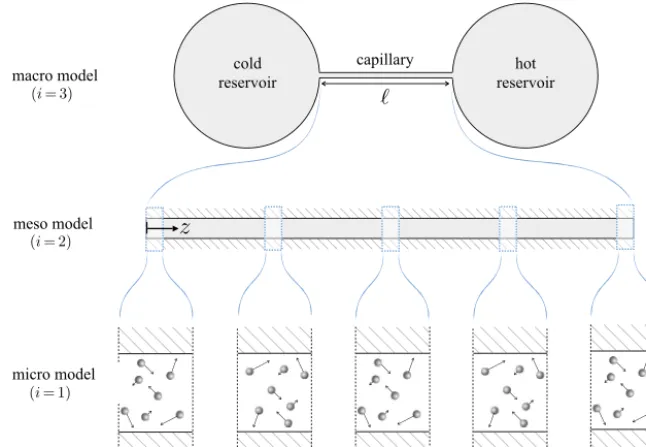
6. Example4:AKnudsencompressor

Finally, weconsider therarefiedgas flowbetweentwo reservoirs, heldatdifferent temperatures,connectedby athin cylindricalcapillary:asingle-stageKnudsencompressor,seeFig. 10.Rarefactioneffectsinthecapillarytransportgasfrom the cold to the hot reservoir; thiscounter-intuitive phenomenon is thermal transpiration(sometimes known asthermal creep)andwasfirstobservedbyReynolds[13].TheconfigurationshowninFig. 10wasconstructedbyRojas-Cárdenasetal. [14] inordertostudythetransientbehaviourofthermaltranspirationinaclosedsystem;someoftheirexperimentaldata ispresentedbelow.

In terms ofsimulation, thissystemcannot be modelled usingstandard Navier–Stokes equationsand boundary condi-tions, sincethermaltranspirationisathermodynamicnon-equilibriumphenomenon[15,16].Ontheother hand,anaccurate gas-kinetictreatmentwouldbecomputationalintractableovertheentiredomain.Totacklethis,wedecomposethesystem intothreecoupledmodels,applyingtheappropriatemodellingassumptionstoeach:thereservoirmodel(macro,i

=

3);the capillarymodel(meso,i

=

2);andthegas-kineticmodel(micro,i

=

1);seeFig. 10.Themacromodeldefiningthereservoir pressuresisobtainedfrommassconservationandbyassuminganidealgas:

dpc

dt3

= −

R

θ

c

Vc

˙

m(z=0)

,

dph

dt3

= −

θ

h

θ

c Vc Vh

dpc

dt3

,

(21)

where pispressure,

R

isthegasconstant,

θ

istemperature, V isthereservoirvolume,m

˙

isthemassflowratealongthe capillary,zisdistancealongthecapillaryfromthecoldtohotreservoir,andthesubscriptsc andhdenotethecoldandhot reservoirs,respectively.Note,hereweassumethatthereisnosignificantchangeinmassofgaswithinthecapillary,though thiscaneasilybeaccountedforifnecessary.

The meso modelforthehigh-aspect-ratio capillaryisobtainedfromthe continuityequation integratedoverthe cross section:

∂

p

∂

t2

+

R

θ

A

∂

m

˙

∂

z

=

0

,

(22)

where A is the cross-sectional area of the capillary. The meso model is coupled to the macro model by the boundary conditions: p

=

pc, m

˙

= ˙

m(z=0) at z

=

0; and p

=

ph at z

=

, where is the length of the capillary. The temperature variationalongthecapillaryisprescribed(usingthesamefitasinRojas-Cárdenasetal.[14])by

θ

=

θ

c

+

(θ

h

−

θ

c

)

eαz

−

1

eα

−

1

,

(23)

where

α

isaconstant.

Themicromodel,

G

,providesameanstoclosetheentiresystem,byrelatingmassflowratetopressureandtemperature:

∂

m

˙

∂

t1

=

G

∂θ

∂

z

;

∂

p

∂

z

;

X

[image:10.561.109.432.56.279.2]

Fig. 10.Schematic of a multiscale simulation strategy for the single-stage Knudsen compressor experimental configuration of Rojas-Cárdenas et al.[14].

where

X

containsinformationregardingthemolecularstructureofthegas,whichisrequiredtoaccuratelymodelthermal transpiration. Here,themicro model

G

isa spatially-distributedarray oflow-variance deviationalsimulation MonteCarlo (LVDSMC)subdomains(seeFig. 10).LV-DSMCisaparticularlyaccurateandlownoisemethodforsimulatingsmalldeviations fromequilibriuminrarefiedgasflows[17,18].Usingmicroparticle-simulationsubdomainstorepresentpointsinthemeso domain is substantially more efficient than modelling the entire channel with a single particle simulation – thisis an applicationof the Internal Multiscale Method (IMM),and readersare referred to [19–21] fora detailed description.The simulatedparticles of each (streamwise periodic)subdomain are forcedby an effectivebody force, which representsthe equivalentpressureandtemperaturegradientoccurringatthatlocationinthemesomodel(thepressureandtemperature arealsoset).Themicromodelisthuscoupledtothemesomodelbythestreamwisepressuregradient,pressure,andmass flowrateateach ofthesubdomainlocations.Forthesimulationswe presenthere, 12subdomainsareused.Foraccuracy, thederivatives inz featuringin Eqs.(22)and(24)are evaluated fromaChebyshev polynomialinterpolation of p andm

˙

fromsubdomainlocationscorrespondingtoChebyshev–Gauss–Lobattopoints.

Viscousdevelopmentwithinthecross-sectionofthecapillarydefinesthecharacteristictimescaleofthemicromodel

T1

=

ρ

R2_cap

μ

,

(25)

where Rcap isthe capillaryradius and

ρ

and

μ

are the average initial densityandviscosity ofthe gas.If we assume a

quasi-steadyvelocityprofile(whichisonlyvalidfort

T1),characteristictimescalesofthemesoandmacromodelcanbe

estimatedfromEqs.(22)and(21),respectively:

T2

=

μ

2

p R2cap

,

(26)

and

T3

=

μ

Vt p R4

cap

,

(27)

wherepistheaverageinitialpressureandVt isthetotalvolumeofthecombinedreservoirs.

TheexperimentsofRojas-Cárdenasetal.[14]wereperformedwithArgongas,aborosilicate(glass)capillaryofcircular cross-sectionwith

=

52

.

7

±

0

.

1 mm,Rcap

=

242

.

5

±

3 μm connectingtworeservoirsofvolume Vc

=

19

.

81

±

0

.

54 cm3and

Vh

=

14

.

85

±

0

.

40 cm3,heldat

θ

c

=

301 K and

θ

h

=

372 K. Aheater appliedtothehotreservoirgeneratedatemperature distribution throughthe capillaryfittedby Eq. (23), with

α

=

84

.

82 m−1.Initially, thetwo reservoirs were held atfixed pressure(p

=

237

.

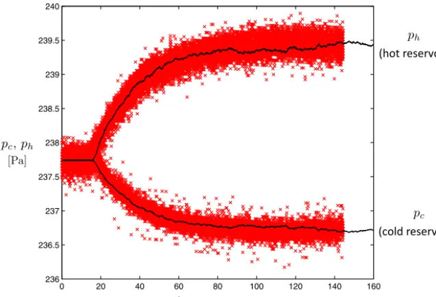
7 Pa),allowing thermaltranspirationflowtodevelop;thesystemwas thenclosed,andthepressurein thetworeservoirsallowedtoequilibrate.Note,inagasthatisnon-rarefiedtheinitialstatewouldbetheequilibriumone.

[image:11.561.117.436.55.272.2]

Fig. 11.Comparisonofexperimentaldataandthemultiscalesolution,fortransientdevelopmentofaKnudsencompressor;aplotofreservoirpressures versustime.Bothreservoirsareheldataconstantpressureuntilapproximatelyt3=18 s,atwhichpointthereservoirsareinstantaneouslyclosedtothe

[image:11.561.137.413.318.538.2]

environment.ExperimentaldataofRojas-Cárdenasetal.[14](×)andthemultiscalesimulation(—).

Fig. 12.Reservoir pressure versus time for increasing values ofStol: 10 (· · ·); 20 (– –); 30 (–·–); 40 (—).

Fig. 11showsthetransientresponseofthepressureineachreservoirafterthesystemisinstantaneouslyclosed;thereis verycloseagreementbetweentheexperimentalmeasurementsandthemultiscalesimulation.Theasymmetryofthefigure around theinitial pressureis causedbythe differentreservoirvolumes(Vc

>

Vh).The multiscaleresultisobtainedwith

Stol

=

10, andrequired theuse oftwelve Intel Xeon X56502.66GHz coresfor 4.13hours (wall-clock time).If thetime

stepsweresetequal(i.e.aconventionalsynchronouscoupling)thesimulationwouldhavetakenover20yearsonthesame hardware. Infact, thesavingover conventionalmodellingis fargreater thanthis, ifwealso takeinto accountthesaving duetospatialmultiscalingbyusingtheIMM[19–21].

Fig. 12 showstheimpactofincreasing Stol;asimilarresultisobtainedinallcases,butwithlowernoiseathigherStol.

This highlights an important generallimitation of multiscalingwith stochastic models (e.g.LVDSMC) orinherently noisy methods (e.g. Molecular Dynamics): fewer timesteps means lesssampling, and thus morenoise. The trade-off inhybrid (continuum-particle)multiscalingcanthusbesummarised:

7. Discussionandsummary

Inthispaper wehave described howan asynchronous couplingofmultiplemodels can beused to balancefine-scale accuracywithlongtimescalepredictionsinscale-separatedsystems.Aphysicalapproximationismadethatrepresentsthe scale separatedsystemby one thatis less, butstill tosome extent,scale separated. Inthe examples presented,we have beenabletomakeverylargecomputationalsavingswithverylittlereductioninmacro-scaleaccuracy.

Inthemajorityoftheseexamples,ithasbeenpossibletoidentifyclearcharacteristictimescales,upon whichtimestep sizesforeachmodelarethen based.Inmanypracticalcases,though,suchidentificationwillnotbestraightforward. Mul-tiple time scales willbe present, andheavy relianceon crudeestimation willbe necessary. In thesecases,performing a dependencystudyon Stolisessentialforobtainingreliablepredictions.

Applyingthe schemetosets ofmodelsthat,despitehavingdisparatecharacteristictimescalesinisolation, arestrongly nonlinearly coupled, presents another issue (e.g. chaotic systems). These systems can demonstrate extreme macro-scale sensitivitytosmallscale fluctuations(i.e. arenot separable).Here,again, theminimumtestofsolution integritymust be thattheresultsareindependentbeyondathresholdStol.

Significantfuturetechnicaldevelopmentneedsaretowardscopingwithsystemsexhibitingtime-varyingdegreesofscale separation.Afullyadaptiveandautomatedscheme–onewhichdoesnotrelyonthepredictionofcharacteristictimescales ofmodels–isthenextmajorstepforward.

Acknowledgements

Thisworkis financiallysupported byEPSRCgrants EP/I011927/1,EP/K038664/1,andEP/K038621/1.Theauthorswould liketothank:MarcosRojas-Cárdenas,IrinaGraur,PierrePerrier,andJ.GilbertMéolansforprovidingtheirexperimentaldata; NicolasHadjiconstantinouforprovidingtheLVDSMCsourcecode;andCarlosDuque-Dazaforthesuggestiontoconsiderthe Lotka–Volterraequationsasanexample.

Appendix A. ParametersforsimulationsofSection5

R

=

10 cm;

air

=

1 μm;

wat

=

0

.

1 mm;

μ

air

=

18

.

6

×

10−6 kg m−1s−1;

μ

wat

=

8

.

9

×

10−4 kg m−1s−1;

ρ

air

=

1

.

23 kg m−3;

ρ

wat

=

1000 kg m−3;

ρ

cyl

=

1

.

23 kg m−3; L

=

1 m; I

=

1

.

26 kg m2; f

=

1

.

59 mHz; A

=

1 Nm;

t1,max

=

T1

/

200;

t2,max

=

T2

/

200;

t3,max

=

T3

/

400.

Appendix B. ParametersforsimulationsofSection6

=

52

.

7 mm;Rcap

=

242

.

5 μm;Vc

=

19

.

81 cm3;Vh

=

14

.

85 cm3;

θ

c

=

301 K;

θ

h

=

372 K;

α

=

84

.

82 m−1;p

=

237

.

7 Pa;

T1

=

9

.

907 μs;T2

=

4

.

205 ms;T3

=

47

.

03 s;

t1,max

=

8

×

10−9 s (setbybest-practiceguidelinesforLV-DSMC);

t2,max

=

T2

/

100;

t3,max

=

T3

/

100;12independentLV-DSMCsubdomainsare positionedonaLobattogridalongthecapillary;On

average

∼

10,000deviationalparticlesareusedpersubdomain.Purelydiffusereflectionisassumedatwalls.AVariableHard Sphere(VHS)modelofArgonisused;VHS diameter

=

4

.

17

×

10−10m;VHS mass

=

6

.

634

×

10−26kg.

References

[1]W.E,B.Engquist,X.Li,W.Ren,E.Vanden-Eijnden,Heterogeneousmultiscalemethods:areview,Commun.Comput.Phys.2(2007)367–450. [2]M.Kalweit,D.Drikakis,Multiscalesimulationstrategiesandmesoscalemodellingofgasandliquidflows,IMAJ.Appl.Math.76(2011)661–671. [3]K.M.Mohamed,A.A.Mohamad,Areviewofthedevelopmentofhybridatomistic-continuummethodsfordensefluids,Microfluid.Nanofluid.8(2010)

283–302.

[4]M.K.Borg,D.A.Lockerby,J.M.Reese,Fluidsimulationswithatomisticresolution:ahybridmultiscalemethodwithfield-wisecoupling,J.Comput.Phys. 255(2013)149–165.

[5]W.E,W.Ren,E.Vanden-Eijnden,Ageneralstrategyfordesigningseamlessmultiscalemethods,J.Comput.Phys.228(2009)5437–5453.

[6]D.A.Lockerby,C.A.Duque-Daza,M.K.Borg,J.M.Reese,Time-stepcouplingforhybridsimulationsofmultiscaleflows,J.Comput.Phys.237(2013) 344–365.

[7]R.Goodwin,AGrowthCycle–Socialism,CapitalismandEconomicGrowth,C.H.Feinstein(Ed.),CambridgeUniversityPress,1967.

[8]V.Volterra,Variationsandfluctuationsofthenumberofindividualsinanimalspecieslivingtogether,J.Cons.- Cons.Perm.Int.Explor.Mer3(1926) 3–51.

[9]A.J.Lotka,Contributiontothetheoryofperiodicreactions,J.Phys.Chem.14(1910)271–274.

[10]R.J.Daniello,N.E.Waterhouse,J.P.Rothstein,Dragreductioninturbulentflowsoversuperhydrophobicsurfaces,Phys.Fluids21(2009)085103. [11]M.A.Samaha,H.V.Tafreshi,M.Gad-el-Hak,Influenceofflowonlongevityofsuperhydrophobiccoatings,Langmuir28(2012)9759–9766. [12]B.Bhushan,Y.C.Jung,K.Koch,Self-cleaningefficiencyofartificialsuperhydrophobicsurfaces,Langmuir25(2009)3240–3248.

[13]O.Reynolds,Oncertaindimensionalpropertiesofmatterinthegaseousstate.PartsIandII,Philos.Trans.R.Soc.Lond.170(1879)727–845. [14]M.Rojas-Cárdenas,I.Graur,P.Perrier,J.G.Méolans,Time-dependentexperimentalanalysisofathermaltranspirationrarefiedgasflow,Phys.Fluids25

(2013)072001.

[15]M.Gad-el-Hak(Ed.),MEMS:IntroductionandFundamentals,CRCPress,2005.

[16]J.M.Reese,M.A.Gallis,D.A.Lockerby,Newdirectionsinfluiddynamics:non-equilibriumaerodynamicandmicrosystemflows,Philos.Trans.R.Soc., Math.Phys.Eng.Sci.361(2003)2967–2988.