Bayesian inference for nonlinear structural time series models

Manuscript version: Author’s Accepted Manuscript

The version presented in WRAP is the author’s accepted manuscript and may differ from the published version or Version of Record.

Persistent WRAP URL:

http://wrap.warwick.ac.uk/63221

How to cite:

Please refer to published version for the most recent bibliographic citation information. If a published version is known of, the repository item page linked to above, will contain details on accessing it.

Copyright and reuse:

The Warwick Research Archive Portal (WRAP) makes this work by researchers of the University of Warwick available open access under the following conditions.

© 2014 Elsevier. Licensed under the Creative Commons Attribution-NonCommercial-NoDerivatives 4.0 International http://creativecommons.org/licenses/by-nc-nd/4.0/.

Publisher’s statement:

Please refer to the repository item page, publisher’s statement section, for further information.

Bayesian Inference for Nonlinear Structural Time Series

Models

Jamie Hall

School of Economics University of New South Wales

[email protected]

Michael K. Pitt

Economics Department University of Warwick [email protected]

Robert Kohn

School of Economics University of New South Wales

[email protected]

September 5, 2012

Abstract

This article discusses a partially adapted particle filter for estimating the likelihood of nonlinear structural econometric state space models whose state transition density cannot be expressed in closed form. The filter generates the disturbances in the state transition equation and allows for multiple modes in the conditional disturbance dis-tribution. The particle filter produces an unbiased estimate of the likelihood and so can be used to carry out Bayesian inference in a particle Markov chain Monte Carlo framework. We show empirically that when the signal to noise ratio is high, the new filter can be much more efficient than the standard particle filter, in the sense that it requires far fewer particles to give the same accuracy. The new filter is applied to several simulated and real examples and in particular to a dynamic stochastic general equilibrium model.

Keywords: DSGE model; Multi-modal; Partially adapted particle filter; State space model

1

Introduction

For a general state space model the standard particle filter (Gordon et al., 1993) gives an unbiased estimate of the likelihood. Andrieu et al. (2010) show that it is possible to use this unbiased estimate within a Markov chain Monte Carlo (MCMC) sampling scheme to carry out Bayesian inference for the parameters of the state space model. They call such a sampling scheme particle MCMC (PMCMC). PMCMC is particularly useful for Bayesian

inference when the state space model is nonlinear or non-Gaussian so that the Kalman filter cannot be used. However, when the signal to noise ratio of the model is high, i.e., when the observation vector gives a very informative measurement on some combination(s) of elements of the state vector, the standard particle filter becomes a computationally inefficient importance sampler (see Pitt and Shephard (1999)).

For many models, this problem can be solved by using adapted particle filters as in Pitt and Shephard (1999), which are more efficient as importance samplers. In addition, Pitt et al. (2012) show empirically that fully adapted particle filters used within PMCMC may require far fewer particles than the standard particle filter to achieve the same accuracy.

While using adapted particle filters can be much more efficient than the standard particle filter, most adapted particle filters require that we can evaluate the state transition density. In important cases, this density is not easily available in closed form. This applies, in particular, to dynamic stochastic general equilibrium (DSGE) models, which are currently widely used in applied macroeconomics. This is in contrast to the standard particle filter which only requires that we can evaluate the observation density and simulate from the state transition density.

Our article proposes to solve this problem by using a partially adapted particle filter that generates the states by first generating the disturbances in the state transition equation. The idea that a stochastic process may become more tractable when considered in terms of its innovations has a long history (see Heunis (2011)). We employ it here because it provides a simple and useful solution to the problem described above. This approach has also been considered in recent independent work by Murray et al. (2012), who use it to estimate biological models with intractable transition densities. Our approach differs in its emphasis on solutions tailored for structural econometrics. Specifically, we demonstrate that a proposal based on a numerical optimisation algorithm and allowing for multiple modes in the disturbances by using mixtures, delivers large efficiency gains when applied to rational-expectations models with high signal-to-noise ratios when compared to the standard particle filter and the filter in Murray et al. (2012). In Murray et al. (2012), the authors use a sigma-point approximation to the conditional densities of the disturbances.

Two other possible improvements to the particle filter for rational expectations models have been proposed in recent literature. Amisano and Tristani (2010) demonstrate that the particle filter can be made more efficient if the proposal distribution for the state vector

xt is conditioned on the first two moments of xt−1, estimated from the particle swarm in

the previous period. Second, Andreasen (2011) demonstrates an improvement when the proposal density for each particle is based on a central-difference Kalman filter with a rescaled covariance. While these contributions are valuable, we believe that the algorithm discussed here represents something of an improvement on these methods, since it is able to deliver results using a relatively small number of particles.

models: specifically, a neoclassical growth model and a consumption-based asset pricing model. Section 5 concludes.

2

Auxiliary Disturbance Particle Filter

This section discusses a particle filter which is effective for certain classes of models explored in this paper. This filter, which we call the auxiliary disturbance particle filter (ADPF), is similar in principle to the auxiliary particle filter but works by sampling the disturbances in the state equation rather than the states themselves. More specifically, while the auxiliary particle filter works by building an approximation to the joint density of (xk_t−1, xt)0, given the previous observationsy1:t−1={y1, ..., yt−1}andyt, the ADPF builds an approximation

to (xk_t−1, ut)0, giveny1:t, whereutis the disturbance term in the state equation. To simplify the notation in this section, we often omit to show dependence on unknown parameters.

2.1 General principles

Consider the state space model with measurement density p(yt|xt) and state transition equation

xt=h(xt−1, ut), (1)

where ut is an independent sequence, h(xt−1, ut) is a nonlinear function of xt−1 and

ut. Given a sample y1:T = {y1, . . . , yT}, and the unknown parameters, the likelihood is p(y1:T) = p(y1)QTt=2p(yt|y1:t−1). When the function h(·) is nonlinear, it is usually

im-possible to evaluate the likelihood exactly, but we can estimate it using one of a number of particle filters. The standard particle filter (Gordon et al., 1993) can be used whenever it is possible to evaluate the measurement densityp(yt|xt) and generate from the state transi-tion equatransi-tion (1). However, the standard particle filter can be quite inefficient in the sense that it produces a likelihood estimate with a large variance compared to more sophisticated particle filters (see Pitt et al., 2012). Pitt and Shephard (1999) suggest a class of auxiliary particle filters that can be much more efficient than the standard particle filter, but most of these require the evaluation of the density of the state transition equation. However, for many cases that are of interest to us, it is infeasible to evaluate the state transition equation density which means that existing auxiliary particle filters cannot be used.

The ADPF attempts to overcome this problem by approximating the state space model with measurement density p(yt|xt) and state transition equation (1) as follows. Suppose that the densityg(yt+1|xt) approximatesp(yt+1|xt) and the densityg(ut+1|yt+1, xt)

approx-imates the densityp(ut+1|yt+1, xt) and that we can evaluatep(yt+1|xt) andg(ut+1|yt+1, xt) and generate fromg(ut+1|yt+1, xt). The choice of this approximate density may be model-specific, although we discuss a general implementation in Section 3.2.

is a swarm of particles generated from an approximation top(xt|y1:t), so thatxkt has asso-ciated weightπ_tk. Now, define

b

p(dxt|y1:t) = N

X

k=1

π_tkδ_xk t(dxt)

whereδs(dx) is the Dirac delta distribution centered ats. We shall show how to construct

b

p(dxt+1|y1:t+1).

Suppose we wish to estimate E(m(xt+1)|y1:t+1), where m(·) is a function of xt+1,

as-suming that the expectation exists. Define the functional

Jt+1(m) = Z

m(xt+1)p(yt+1|xt, ut+1)p(xt, ut+1|y1:t)dxtdut+1,

=

Z

m(xt+1)p(yt+1|xt, ut+1)p(ut+1)p(xt|y1:t)dxtdut+1,

=

Z

m(xt+1)p(yt+1|xt)p(ut+1|yt+1, xt)p(xt|y1:t)dxtdut+1, (2)

using the identityp(yt+1|xt, ut+1)p(ut+1) =p(yt+1|xt)p(ut+1|yt+1, xt). Then, it is straight-forward to check thatE(m(xt+1)|y1:t+1) =Jt+1(m)/Jt+1(1), where 1 is the unit function,

and p(yt+1|y1:t) =Jt+1(1).

We approximate Jt+1(m) by replacing p(xt|y1:t)dt in (2) bypb(dxt|y1:t) to obtain,

Jt+1(m)≈ Z

m(xt+1)p(yt+1|h(xt;ut+1))p(ut+1)bp(xt|y1:t)dut+1dxt

=

Z

m(xt+1)

p(yt+1|h(xt;ut+1))p(ut+1)

g(ut+1|yt+1, xt)g(yt+1|xt)

g(yt+1|xt)g(ut+1|yt+1, xt)pb(dxt|y1:t)dut+1

= N

X

i=1

ωi_t|t+1

! Z

m(xt+1)

p(yt+1|h(xt, ut+1)p(ut+1)

g(ut+1|yt+1, xt)g(yt+1|xt)

g(ut+1|yt+1, xt)bgN(dxt|y1:t+1)dut+1

where

b

gN(dxt|y1:t+1) =

N

X

k=1

π_tk_|t+1δ_xk

t(dxt), π

k t|t+1 =

ω_tk_|t+1

PN

i=1ωti|t+1

with ω_tk_|t+1 =g(yt+1|xkt)πtk.

Suppose thatuk

t+1 ∼g(ut+1|yt+1, xkt) and xkt+1=h(xkt, ukt+1), and put

ωk_t+1 = p(yt+1|x k

t+1)p(ukt+1)

g(uk

t+1|yt+1, xkt)g(yt+1|xkt)

, π_tk₊₁ = ω k t+1 PN

i=1ωti+1

We obtain the estimate

b

Jt+1(m) =

N

X

i=1

ωi_t|t+1

! _N

X

i=1

ωi_t+1

! _N

X

k=1

m(xk_t+1)πk_t+1 (3)

with Jb_t+1(1) =

N

X

i=1

ωi_t|t+1

! _N

X

i=1

ωi_t+1

!

, (4)

so that

b

E(m(xt+1)|y1:t+1) =

N

X

k=1

m(xk_t+1)π_tk₊₁ and p_b(yt+1|y1:t) = N

X

i=1

ωi_t|t+1

! _N

X

i=1

ωi_t+1

!

.

This suggests that we take {(xk_t+1, π_tk₊₁), k = 1, . . . , N} as the swarm of particles that we use to approximate p(xt+1|y1:t+1) and define

b

p(dxt+1|y1:t+1) =

N

X

k=1

π_tk₊₁δ_xk

t+1(dxt) .

The following algorithm formally describes the ADPF and is initialized with a sample

xk₀ ∼p(x0) with massπ0k= 1/N fork= 1, ..., N.

Algorithm 1. For t =0, ..,T −1 , given samples xk_t ∼ p(xt|y1:t) with mass πkt for k =

1, ..., N.

1. Fork= 1 :N,computeω_tk_|t+1=g(yt+1|xkt)πtk, πkt|t+1 =

ωk t|t+1

PN i=1ωit|t+1

.

2. Fork= 1 :N,samplex_ek_t ∼PN

i=1πit|t+1δxi t(dxt).

3. Fork= 1 :N,sampleuk_t+1 ∼g(ut+1|xe

k

t;yt+1) and put xkt+1=h(xkt;ukt+1).

4. Fork= 1 :N,compute

ωk_t+1 = p(yt+1|x k

t+1)p(ukt+1)

g(yt+1|ex

k

t)g(ukt+1|xe

k t;yt+1)

, π_tk₊₁= ω k t+1 PN

i=1ωit+1

.

The estimate of the likelihood corresponding to the ADPF is

b

p(y1:T) = T Y t=1 N X i=1

ω_ti_−1|t

! _N

X

i=1

ω_ti

!

By Andrieu et al. (2010)) we can write this estimate of the likelihood as pbN(y1:t|θ, ζ)

whereζ consists of a set canonical random variables that are used to construct the estimate and that have density pN(ζ). Without loss of generality we can assume that elements of

ζ are uniform independent random variates. The estimated likelihood also depends on the number of particles N.

Theorem 1. The estimatepbN(y1:T|ζ) is unbiased in the sense that

Z

b

pN(y1:t|ζ)pN(ζ)dζ=p(y1:T).

The proof is in Appendix A.

3

Particle filter performance on a first order nonlinear

au-toregressive model

3.1 The model

Consider the following univariate nonlinear time series model,

yt=xt+σεεt (6)

xt=φxt−1+σu ut+δu2t

(7)

whereεtand ut areiid standard normal random variables. We choose this model because it is one of the simplest nonlinear extensions to a well-understood linear model. Whenσε is small it is also one of the simplest examples of the class of structural economic models that we consider below. The parameterδ controls the degree of nonlinearity in the model; withδ= 0 the model is a first order autoregressive (AR(1)) model with observation noise. Whenδ exceeds about 0.5, the behavior of the model becomes noticeably different to that of a linear model. For a comprehensive analysis of this general class of models, see Aruoba et al. (2011).

3.2 ADPF implementation and testing

We choose a normal distribution with mean φxt−1 +σuδ and variance σ2ε +σu2(1 + 2δ2) for the approximating density g(yt|xt−1) because it matches the first two moments of

yt, conditional on xt−1. To estimate g(ut|yt, xkt−1), we proceed as follows. Let `k(u) =

logp(yt|u, xkt−1)φ(u; 0,1) for given xkt−1 and yt, where φ(u;a, b2) is the univariate normal

φ(u;u_ek

t,∆kt) to `k(u), where ∆tk =− ∂2`k(u)/∂u2

−1

evaluated atu =u_ek

t. Appendix B gives more details on the optimization procedure used here, and in the next example.

The normal approximation must be renormalised to adjust for the presence of multiple local modes. Multiple modes occur because the law of motion is a nonlinear polynomial, so that `k(u) is also nonlinear; in this case, a quartic equation. In other words, a given observation ytmight have been generated by more than one possible value of ut. For that reason, a simple normal approximation is inadequate. To see this, consider the limit as

σε→0. In this case, the model becomes deterministic, and almost any realised level of yt is then consistent with two values ofut. Suppose, in a particular case, we label those two values u(1)_t and u(2)_t . The algorithm, as described so far, would place a mass of 1 on the value ofutthat the numerical minimiser found; that is, if it happened to find the first mode, it would sample ut from g(ut|yt, xkt) = φ(ut;u

(1)

t ,∆

(1)

t ), where ∆

(1)

t =− ∂2`k(u)/∂u2

−1

evaluated atu=u(1)_t .

Figure 1 illustrates this point. The left-hand panel plots xt as a function of ut, that is, equation (7). This plot is assumes a previous value xt−1 = 0, and parameter values

δ = 0.5, σε = 0.2, σu = 1. Any value of the underlying state xt>−0.5 is consistent with two possible values of ut. For example, a value of xt = 0.5 could have been generated by ut ≈0.41 or ut ≈ −2.4. The right-hand panel plots an unnormalised version of `k(u), conditional on an observation yt = 0.5. The distribution is obviously bimodal; with the noise varianceσε small in this case, the two modes of `k(u) are close to 0.41 and−2.4.

Withσε →0, the simple maximisation approach described above would place a weight of 1 on, say, the value of u= 0.41, ignoring the other possibility. This is not an accurate approximation to the true p(ut|yt, xkt)), and will produce what appears to be a biased estimate of the log-likelihood. Although the ADPF is unbiased no matter what proposal densityg(ut|yt, xkt−1) is used, in cases with a high signal to noise ratio, a very large number

of particles are required to counteract the problem described in the text, which defeats the purpose of using the filter. Instead, a better approximation is given by the mixture density

g(ut|yt, xkt) =φ(u

(1)

t ; 0,1)φ(ut;u

(1)

t ,∆

(1)

t ) +φ(u

(2)

t ; 0,1)φ(ut;u

(2)

t ,∆

(2)

t ). (8) In this simple model, it is feasible to search for both modesu(1)_t and u(2)_t , but we develop a more general approach, with the goal of constraining the required computation time as the dimension of the model increases. Given a set of estimatesue

k

t, obtained as described above, we form a proposal density for each disturbance uj_t, j = 1, . . . , N, by taking an equally-weighted mixture of those u_ek that generate a value foryt within 3 standard deviations of the observed value. That is,

g(uj_t|yt, xjt)∝ N X i=1 χ  

yt−φxj_t−1−σu uit+δ(uit)2

σε

!2

≤32



φ

whereχ[ω] is the characteristic or indicator function of eventω. This takes advantage of the fact that values ofxk_t−1 tend to be clustered, so that a value of_euk_t found for a particular

xk_t−1 has a good chance of working well for another xj_t−1, in the sense of implying a mean value ofyt close to the observed one. This method of generating a proposal generalises to more complex models, such as the DSGE example discussed in Section 4 below. Note that the proposal density is reweighted by the true density in step 4 of the ADPF algorithm. Thus, there is no need to ensure that (for instance) the proposal density puts the correct mass on different possible values of u, as in equation (8). All that is required is that each possible value ofu has a reasonable chance of being used in the proposal.

Figure 1 about here

We performed a simulation study to compare the performance of the ADPF with the standard SIR particle filter and the ‘CUPF1’ algorithm described in Murray et al. (2012). That algorithm has a similar structure to the ADPF, except that the first-stage proposal density g(yt|xkt−1) and the second-stage density g(ukt|yt, xkt−1) are both given by the

Un-scented Kalman Filter (Wan and van Der Merwe, 2000), run individually for each particle. We briefly describe the Unscented Kalman Filter, with a full description given by Wan and van Der Merwe (2000) and van Der Merwe et al. (2001). In the Unscented Kalman Filter the prior meanxt−1 is propagated through the model’s law of motion, along with a

set of ‘sigma points’xt−1± p

λPt−_1(i), wherePt−1 is the prior state covariance augmented

with the covariance of the disturbances and noise terms,λis a parameter of the algorithm, √

· denotes a matrix square root, and P_(i) is the ith row of the matrix.1 After the sigma points are propagated through the law of motion and the observation equation, we obtain an accurate estimate of the mean and covariance of the state and disturbances, conditional on the observation yt.

We evaluated the filters on four different parameter settings: with either δ = 0.7 (a high nonlinearity case) or δ = 0.1 (low nonlinearity), and with either σe = 0.01 (a high signal to noise (SNR) ratio) orσe= 1.0 (low SNR). In all cases, we setσu = 1 andφ= 0.6. For each test, we simulated a single dataset of 50 observations. We chose this number of observations because it roughly corresponds to the length of a quarterly macroeconomic data series. Using 1000 replications, we calculated the median log-likelihood estimated by the filters on each dataset, along with the interquartile range of their estimates, as well as the standard deviation of their log-likelihood estimates. Additionally, we used a standard particle filter with 1,000,000 particles to estimate the true value of the loglikelihood, which we used to estimate the bias of the loglikelihood estimates of the other filters.

1

More precisely,λis a function of parameters α,β andκ. We used the values suggested in Wan and van Der Merwe (2000), namelyα= 10−3_{,β= 2,κ= 0. We experimented with different values, but found}

3.3 Results

The performance of the ADPF is comparable to that of the standard SIR filter in the two cases with low single-to-noise ratio. In both scenarios, the standard deviation of the log-likelihood estimates from the ADPF with 50 particles is between those from the standard particle filter with 100 and 500 particles. This is similar to the performance of the fully adapted particle filter, which makes no substantial improvement on the standard particle filter when the signal to noise ratio is relatively low.

The situation is different with a high SNR, reported in Tables 1 and 2. In these cases, the ADPF proposal draws fromp(ut|yt, xt−1) are much more useful than the draws from the

proposalp(xt|xt−1) used by the standard particle filter, because the observationytis highly informative about the current position ofxt(and therefore ofut). As a result, the precision of the ADPF with 50 particles is similar to the standard particle filter’s with more than 7500 when the model is markedly nonlinear, and more than 15000 in the approximately linear case. Additionally, the CUPF1 variation does not appear to be well adapted to this class of model, perhaps because more than the first two moments are required for a good approximation to the target density.

Tables 1 and 2 about here.

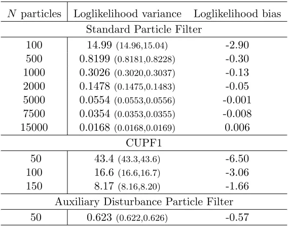
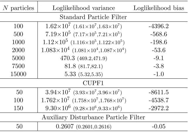
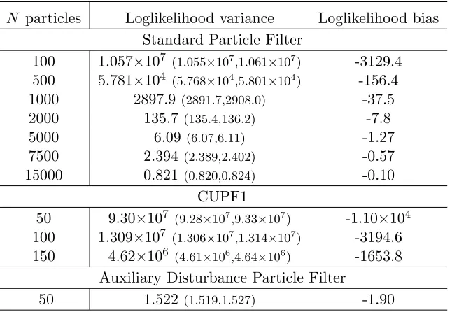
Tables 3 to 6 report the estimated bias and variance in the log-likelihood estimates for the four combinations of nonlinearity and signal to noise ratio. The asymptotic anal-ysis in Pitt et al. (2012) suggests that the log-likelihood estimates should have a bias approximately equal to −0.5 times their variance, and that the variance should decrease in proportion to the number of particles used. Our simulations of the simple quadratic AR(1) model are broadly consistent with these expectations, with the predictions borne out well in the low signal to noise ratio cases. The high signal to noise ratio cases reported in Tables 5 and 6 appear to be consistent with the predictions of Pitt et al. (2012) as the number of particles becomes large, though the uncertainty around these estimates is larger in these cases.

Tables 3 to 6 about here.

4

Parameter estimation

4.1 Example 1: Neoclassical growth model

4.1.1 Model

representative household, which chooses between consumption ct and investment in next period’s capital stockkt. The household’s goal is to maximise discounted lifetime utility, given by

U =

∞

X

t=0

βtlogct

subject to a feasibility constraint,

ct+kt=Atkαt−1+ (1−δ)kt−1 , (10)

whereδ∈[0,1], and a productivity shock

logAt=ρlogAt−1+t t∼N(0, σ2) . (11)

where ρ ∈ (0,1). The solution of the model consists of equations (10) and (11) plus a consumption Euler equation,

c−_t1 =βEt

c−_t+11 αAt+1ktα−1+ 1−δ . (12)

Here, EtX denotes the model-consistent expectation of X, conditional on information available at timet.

This solution can be converted to a Markov process on the assumption of rational expectations as in Klein (2000). If the depreciation rate δ is below one, the conversion cannot be expressed in closed form, and some type of approximation must be used. We chose a second-order approximation, using the methods described in Klein (2000) and Gomme (2011). The output of these methods is a law of motion for the vector xt = (ct, kt, at)0 of the form

xt=d+Ext−1+F t+ I3⊗x0t−1

Gxt−1

+ I3⊗x0t−1

Ht+ I3⊗0t

J t. (13)

The reduced-form coefficient matricesd,E,F,G,H andJ are functions of the structural parameters, but must be calculated numerically as we do not have analytical expressions for them.

As is standard in the DSGE literature, we add the ‘measurement error’νt to the obser-vation equation, in order to avoid stochastic singularity and for computational convenience, i.e.

the model, and the variance of the measurement noise is comparable to that of the in-novations in the model’s law of motion. Here, we maintain the assumption of a high signal to noise ratio, settingσ2_ν to 10−8. We set the rest of the parameters to fairly stan-dard calibrated values (see e.g. Gomme, 2011; Schmitt-Groh´e, 2004). Specifically, we set

β= 0.99, α= 1/3, ρ= 0.8, δ= 0.05 and σ2= 0.022.

4.1.2 Estimation

To evaluate the performance of the ADPF in estimation, we simulated a data series of 50 observations using equations (13) and (14). Again, we chose this length observations because it is of the same order of magnitude as a macroeconomic time-series. We then use the adaptive random walk Metropolis-Hastings (Roberts and Rosenthal, 2001) to take 100,000 draws from the parameter vector. We fix β at 0.99. This is standard, as it is difficult to identify β. The vector of unknown parameters is θ = (α, ρ, δ, σ). Table 7 summarizes the priors on the structural parameters, which are set relatively loosely to assist identification.

Table 7 about here.

We initialised the Metropolis-Hastings chain at the maximum likelihood estimate ob-tained from a first-order approximation of the model via the Kalman filter. We chose this initialisation method because we observed that the standard deviation of the log of the estimate of the likelihood obtained by the ADPF increased significantly in some areas of the support ofθaway from the true values, making it difficult for the Metropolis-Hastings algorithm to converge. Additionally, initialising the MCMC chain in this way has been the practice for second-order DSGE estimation using the standard particle filter, as in Fern´andez-Villaverde and Rubio-Ram´ırez (2008) and Amisano and Tristani (2010). The Metropolis-Hastings proposal covariance matrix was initialised to a diagonal matrix of small positive values, with adaptation beginning after 100 draws.

We repeated this procedure using different numbers of particles in the particle filter and the ADPF (using the same simulated data). For each estimation run, we report the Metropolis-Hastings acceptance rate, the inefficiency, and the computation time. For each component of the parameter vector, the inefficiency is calculated as IF = 1 + 2PL?

j=1ρbj,

where ρ_bj is the estimated autocorrelation of the parameter iterates at lag j. If K is the sample size used to computeρbj, then the maximum lag length is set toL

? _{= min{1000, L},} withL being the lowest indexj such that |ρ_bj|<2/

√

K.

Since the actual wall-clock estimation time depends heavily on the details of a particular implementation, we report instead a measure of computation time calculated as the number of evaluations of the model’s law of motion required to produce one effectively independent draw from a given parameter. Thus, if N particles use the law of motion an average of

the computation time as N ×IF. Here, we ensure a fair comparison with the standard particle filter by penalising the ADPF for the multiple function evaluations required for optimising `k(ut). We estimate k by keeping a tally of the number of times the law of motion subroutine was called during estimation. For this model, the value ofkwas around 16 per particle per observation.

In implementing the ADPF, we use the same approach as in section 3.2. For the first-stage proposal densityg(yt+1|xt), we use a normal distribution matching the first two

moments ofyt+1 conditional onxt, which can be calculated from equations (13) and (14).

Specifically, substituting (13) into (14), dropping the negligible measurement error term

νt, and taking expectations, the mean of yt conditional onxt−1 is

µy,t=d1+E1xt−1+x0t−1G1xt−1+σ2J1 , (15)

whered1 andE1 are the first element and row ofdand E,G1 is the upper 3×3 blocks of

G, andJ1 is the first element of J. Similarly, the conditional variance ofyt is

σy,t=σ2F12+ 2σ2F1x0t−1H1+σ2 x0t−1H1 2

+σ4J₁2 , (16)

where F1 is the first element of F, H1 is the first row of H, and J1 is the first row of J.

Note that if we use a first-order approximation to the solution of the DSGE model, then

G=H =J = 0, and the mean (15) and variance (16) are equal to the one-step prediction mean and variance from the Kalman filter (conditioned on a given value forxt−1).

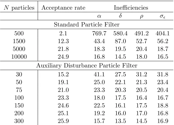
4.1.3 Results and Analysis

As expected, the estimated parameter values from all filters are very similar. However, there are notable differences in efficiency and computing time. Table 8 reports the Metropolis-Hastings acceptance rates for different numbers of particles used in the standard particle filter and the ADPF. It also shows the inefficiencies for each component of the parameter vector. As the number of particles used increases, so that the estimates of the loglikelihood become more precise, the acceptance rate increases. This is true for both the standard particle filter and the ADPF. Broadly speaking, the ADPF performs about as well with 50 particles as does the standard particle filter with several thousand particles. Conversely, to approach the performance of the ADPF with 300 particles, the standard particle filter must use about 10,000.

with around 1,500 particles for the standard particle filter and 30 for the ADPF. The computing time of the ADPF is roughly one fifth of the standard particle filter. Since the implementation of the ADPF leaves scope for optimisation or parallel computing, this relative performance could be improved further in practice.2

Table 5 also shows the variance of each filter’s loglikelihood estimates, evaluated by taking 75 repeated loglikelihood estimates at the true value ofθ. These results are broadly consistent with the asymptotic analysis in Pitt et al. (2012), which suggests that the optimal computing time would be attained when the loglikelihood variance is around 0.81. In the case of the ADPF, the optimal computing times occur when the variance is slightly higher than that. We conjecture that this is because the analysis in Pitt et al. (2012) assumes that a perfect Metropolis-Hastings proposal distribution is available.

Tables 8 and 5 about here.

4.2 Example 2: Asset pricing with habits

4.2.1 The Model

This section demonstrates the full-information estimation of a structural asset pricing model, specifically, a consumption-based model with external habits (Campbell and Cochrane, 1999). Previously, this type of model has been taken to the data by matching moments, e.g. Campbell and Cochrane (1999)), using GMM , e.g. Hyde and Sherif (2005), or a linear approximation, e.g. Bouakez et al. (2005)). Here, we estimate the likelihood directly.

The model assumes that the representative agent’s consumption process is

∆ logCt=g+νt , (17)

whereν ∼N(0, σ2). The agent’s utility function is given by

Ut=Et

∞

X

t=0

βt(Ct−Xt)

1−γ

1−γ , (18)

where Xt is the (external) habit stock, interpreted as the minimum level of consumption required to maintain a well-defined utility (i.e., the household must ensure thatCt> Xt). The surplus consumption ratioStand the deviationestof logStfrom its meanSare defined

by

St=

Ct−Xt

Ct

and s_et= logSt−logS

2_{The optimisation step of the APDF algorithm can be performed in parallel for larger problems.}

Ad-ditionally, we penalise the ADPF for every evaluation of the law of motion; but, conditional onxkt−1, only

The law of motion of est is assumed to be

e

st=φest−1+

1

S

p

1−2est−1−1

νt , (19)

where the disturbanceνt is the same as the consumption innovation in equation (17), and the steady-state level ofSt is

S=σ

r _γ

1−φ . (20)

See Campbell and Cochrane (1999) for discussion of the derivation of equations (19) and (20). The ratio St is stationary, since the level of the habit stock Xt is constructed to grow at the same rate asCt in the long run. The nonlinear functional form for est means

that habit is a slowly-moving average of recent consumption in ‘normal times’ (when the habit stock is close to its mean) but responds more sensitively to consumption innovations during ‘bad times’ (whensetis low). This nonlinearity allows the model to address both the

equity premium puzzle and the risk-free rate puzzle (see Campbell and Cochrane (1999) for further discussion).

On that basis, it can be shown that the equilibrium price-dividend ratio of a financial asset satisfies

Pt

Dt

=βtEt

exp [γ(_est−est+1) + (1−γ)(g+νt+1)]

1 + Pt+1

Dt+1

, (21)

whereβtis the intertemporal discount factor in periodt. This is the Fundamental Theorem of Finance—the current asset price equals the risk-neutral expectation of next period’s asset price and return—using the functional forms implied by equations (18) to (20) (Campbell and Cochrane, 1999). Since not all changes in the typical household’s intertemporal trade-offs can be explained by consumption habits, we choose to perturb this parameter with a shock process that is a random walk in logs,

βt=βebt, bt=bt−1+t , (22)

wheret∼N(0, σ2).

Equations (17), (19), (21) and (22) characterise the model. The observed variables are ∆ logCt and ∆ log_DPt_t, and the observation equations are (17) and (21). We approximate equation (21) using a third-order Taylor series expansion in _es at _es = 0 because it is the simplest approximation that describes the nonlinear behaviour of the price-dividend ratio adequately. Thus equation (21) is approximated as

log Pt

Dt

= Γ0+ Γ1est+ Γ2es 2

t + Γ3es 3

t , (23)

4.2.2 Estimation

We apply the model to observations of growth in the S&P500 price-dividend ratio and US consumption using quarterly observations from 1950 to 2011, a total of 248 datapoints, that are plotted in Figure 2. The S&P500 series is from Shiller (2006), while the consumption series is the seasonally adjusted real personal consumption expenditure series from the Bureau of Economic Analysis (series code PCECC96).

Figure 2 about here

Since it is unlikely that consumption is observed perfectly, we modify equation (17) to include an iid noise term ηt ∼N(0, σ2η). The restrictions placed on the joint distribution of consumption and asset price growth by the structural model allow us to identify this noise term separately from the consumption innovation νt. We use a fairly tight prior distribution to constrain the variance ofηt, because the structural model would otherwise struggle to improve on the assumption that consumption and price-dividend ratio growth are both iid. This exercise is intended to illustrate the ADPF estimation method, rather than provide a precise explanation of intertemporal saving decisions, and while the addition of external habits greatly improves the consumption-based asset pricing model, its chief virtue is still its simplicity, rather than its flexibility.

Table 10 gives the prior distributions of the other parameters. The priors are chosen to ensure that they imply reasonable properties for the risk-free interest rate and consumption. Specifically, we select priors ongandσ_ν2to ensure that the underlying consumption growth series is close in mean and variance to the observed one. More importantly, Campbell and Cochrane (1999) show that the implied level of the risk-free rate is

rf =−logβ+γg−

γ S

2

σ2

2 . (24)

Instead of placing a prior on β directly, we choose a prior for rf that ensures it is a low positive number. Finally, we choose relatively loose priors forγandφ. Table 10 summarises the prior distributions of the parameters, which we assume are mutually independent.

Table 10 about here.

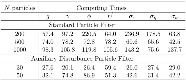
4.2.3 Results and Analysis

Table 11 reports the posterior means and standard deviations (in brackets) of the pa-rameters. Table 12 reports the acceptance rates an and the inefficiency estimates of the parameters. The table shows that the Metropolis-Hastings acceptance rates generally in-crease and the inefficiencies generally dein-crease with a higher number of particles for both the standard particle filter and the ADPF. Broadly speaking, the performance of the ADPF with a given number of particles appears to be comparable to that of the standard particle filter with 15 or 20 times more particles.

Table 13 presents the computing times, calculated in the same manner as described above. Here, a clearer difference emerges between the standard particle filter and the ADPF. The estimated computing times of the ADPF are roughly twice as fast as the standard particle filter’s. In calculating these times, we penalised the use of the analytical derivative of equation (23) equally as heavily as using the law of motion itself. If these analytical derivatives are discounted—as may happen in applications where the derivatives are considerably simpler than the transition equations—the performance of the ADPF is around 5 times better than the standard particle filter’s.

Tables 11, 12 and 13 about here.

Notably, the posterior mean ofrf _{is unchanged from its prior mean. However, despite} the apparently weak identification of this parameter, the nonlinear estimation reveals some amount of information about it. Figure 3 is a scatterplot showing the values ofβ implied by the draws of rf _{against the draws of φ. (The graph shows 1500 randomly-selected} draws from the MCMC chain for the ADPF with 50 particles.) Perhaps surprisingly, a more persistent habit stock (higherφ) is associated with more value placed on the future (higher β). This is in fact consistent with the relationship implied by equation (21). To see this, substitute (19) into (21) and ignore shocks after period t,

Pt

Dt

∝βexp [γ(1−φ)s_et]

1 + Pt+1

Dt+1

,

showing that a rise inβ is, other things equal, associated with a fall in (1−φ).

Figure 3 about here

5

Conclusion

Appendices

Appendix A

Proofs

The proof can be derived from Del Moral (2004) (Section 7.4.2, Proposition 7.4.1). How-ever, we believe that it is easier to follow the proof of Theorem 1 in Pitt et al. (2012) and we do so here. LetAt={(xkt, πtk), k= 1, . . . , N} be the swarm of particles at timet.

Proof of Theorem 1.

E(pbN(yt|y1:t−1)|At−1) =

N

X

k=1

p(yt|xkt−1)πtk−1 (25)

E(pbN(yt−h:t|y1:t−h−1)|At−h−1) =

N

X

k=1

p(yt−h:t|xkt−h−1)πkt−h−1 (26)

E(pbN(y1:t)|A0) =

N

X

k=1

p(y1:t|xk0)π0k (27)

E(pbN(y1:t)) =p(y1:t) (28)

Equations (25) and (26) are obtained as in Lemmas 6 and 7 respectively of Pitt et al. (2012). Equation (27) is obtained by taking h = t−1 in (26) and (28) is obtained from (27) becauseA0={(xk0, πk0), k= 1, . . . , N} withxk0 ∼p(x0) andπk0 = 1/N.

Appendix B

Optimisation Method

While the optimization of`(uk_t|yt, xkt−1) can be performed in many ways, we find that the

Levenberg-Marquardt algorithm (Marquardt, 1963), as implemented by Mor´e et al. (1980), delivers satisfactory results. This algorithm is applied sequentially to each particle at each time step. By default, it uses numerical differentiation to estimate_bg= _∂u∂`

i andAb=

∂2_`

∂ui∂uj.

In the case of the asset pricing model, analytical derivatives are easy to calculate and are used instead. At each step of the iteration, the proposed value of uis

u(i)=u(i−1)−Ab+νI −1

b

g.

The value ofν is initialised at 10, then increased by a factor of 10 if the proposed value is rejected, and decreased by a factor of 10 if the proposed value is accepted. The algorithm is deemed to have converged ifk_bgk<10−3, where k_bgkis the Euclidean norm, or if the sum of squared residuals (scaled by their standard deviations) is less than 10−5_{. The algorithm}

In each case, each component of uk_t is initialised with a draw fromN(0,2) (recall that each u variate is, by construction, standard normal). We made this choice to ensure that the algorithm explores the tails of the distribution with reasonable probability.

Appendix C

Asset Pricing Approximation

Taking a third-order Taylor approximation of equation (21), then evaluating the coefficients withest=est+1 =bt=νt+1 = 0, gives the following values for the Γicoefficients in equation

(23), whereG= exp(g), whereg is the growth rate from equation (17):

Γ0 =

βG Gγ_−βG,

Γ1 =

(1−φ)Gγ+1βγ

(Gγ_−βG)(Gγ_−φβG),

Γ2 =

1 2Γ0Γ1

(1−φ)(Gγ−βG)γ(Gγ+φβG)

βG(Gγ_−φβG) ,

Γ3 =

1 6

(1−φ)3Gγ+1βγ3(G2γ+ 2βφGγ+1+ 2βφ2Gγ+1+β2φ3G2) (Gγ_−βG)(Gγ_−φβG)(Gγ_−φ2_βG)(Gγ_−φ3_βG) .

References

Amisano, G. and Tristani, O. (2010), “Euro area inflation persistence in an estimated nonlinear DSGE model,”Journal of Economic Dynamics and Control, 34, 1837–1858.

Andreasen, M. M. (2011), “Non-linear DSGE models and the optimized central difference particle filter,”Journal of Economic Dynamics and Control, 35, 1671–1695.

Andrieu, C., Doucet, A., and Holenstein, R. (2010), “Particle Markov chain Monte Carlo methods,” Journal of the Royal Statistical Society: Series B, 72, 269–342.

Aruoba, S. B., Bocola, L., and Schorfheide, F. (2011), “A new class of nonlinear time series models for the evaluation of DSGE models,” Mimeo, University of Maryland.

Bouakez, H., Cardia, E., and Ruge-Murcia, F. J. (2005), “Habit formation and the persis-tence of monetary shocks,” Journal of Monetary Economics, 52, 1073–1088.

Del Moral, P. (2004),Feynman-Kac Formulae: Genealogical and Interacting Particle

Sys-tems with Applications, New York: Springer.

Fern´andez-Villaverde, J. and Rubio-Ram´ırez, J. F. (2008), “How Structural Are Structural Parameters?” inNBER Macroeconomics Annual 2007, eds. Acemoglu, D. Rogoff, K. and M., W., University of Chicago Press, vol. 22 of National Bureau of Economic Research

Working Paper Series.

Gomme, P.and Klein, P. (2011), “Second-order approximation of dynamic models without the use of tensors,” Journal of Economic Dynamics and Control, 35, 604–615.

Gordon, N., Salmond, D., and Smith, A. (1993), “Novel approach to nonlinear/non-Gaussian Bayesian state estimation,” Radar and Signal Processing, IEE Proceedings F, 140, 107 –113.

Heunis, A. J. (2011), “The Innovations Problem,” inOxford Handbook of Nonlinear Filter-ing, eds. Crisan, D. and Rozovskii, B., New York: Oxford University Press, pp. 425—49.

Hyde, S. and Sherif, M. (2005), “Don’t break the habit: structural stability tests of con-sumption asset pricing models in the UK,”Applied Economics Letters, 12, 289–296.

Klein, P. (2000), “Using the generalized Schur form to solve a multivariate linear rational expectations model,”Journal of Economic Dynamics and Control, 24, 1405–1423.

Marquardt, D. W. (1963), “An Algorithm for Least-Squares Estimation of Nonlinear Pa-rameters,”SIAM Journal on Applied Mathematics, 431–441.

Mor´e, J. J., Garbow, B. S., and Hillstrom, K. E. (1980), “User Guide for MINPACK-1,” Tech. Rep. ANL-80-74, Argonne National Laboratory, Argonne, IL.

Murray, L. M., Jones, E. M., and Parslow, J. (2012), “On Collapsed State-space Models and the Particle Marginal Metropolis-Hastings Sampler,” Tech. rep.

Pitt, M. K. and Shephard, N. (1999), “Filtering via Simulation: Auxiliary Particle Filters,”

Journal of the American Statistical Association, 94, 590–599.

Pitt, M. K., Silva, R., Giordani, P., and Kohn, R. (2012), “On some properties of Markov chain Monte Carlo simulation methods based on the particle filter,” Journal of

Econo-metrics, in press.

Roberts, G. and Rosenthal, J. S. (2001), “Optimal scaling for various Metropolis-Hastings algorithms,” Statistical Science, 16, 351–367.

Schmitt-Groh´e, S.and Uribe, M. (2004), “Solving dynamic general equilibrium models using a second-order approximation to the policy function,” Journal of Economic Dynamics

Shiller, R. J. (2006),Irrational Exuberance, New York: Currency/Doubleday.

van Der Merwe, R., Doucet, A., de Freitas, N., and Wan, E. A. (2001), “The unscented particle filter,” in Advances in Neural Information Processing Systems 13, eds. Leen, T. K., Dietterich, T. G., and Tresp, V., Cambridge, MA: MIT Press, pp. 584—90.

Wan, E. A. and van Der Merwe, R. (2000), “The unscented Kalman filter for nonlinear estimation,” in Adaptive Systems for Signal Processing, Communications, and Control

-3 -2 -1 1 ut

-0.5 0.5 1.0 1.5

xt

-3 -2 -1 1 ut

-15

-10

-5

{

Figure 1: New statextas a function of shock ut (left) and log-posterior of ut (right) for a realisation of the quadratic AR(1) model

P/D Growth

%

1950 1960 1970 1980 1990 2000 2010

−20

−10

0

10

20

C Growth

%

1950 1960 1970 1980 1990 2000 2010

−2

0

2

4

Figure 3: Bivariate scatter-plot of the MCMC draws ofβ andφfor the asset pricing model

]

N particles Median loglikelihood IQR Median std. dev. Standard Particle Filter

100 -3241.7 2876.8 4028.3 500 -285.8 588.7 847.8 1000 -118.8 500.9 334.4 2000 -80.0 206.9 104.1 5000 -69.6 35.1 21.7 7500 -68.3 37.7 9.0 15000 -67.7 6.4 2.3

CUPF1

50 -7587.2 3203.8 6278.5 100 -3255.3 1881.4 4197.5 150 -1924.8 1278.6 3048.9

Auxiliary Disturbance Particle Filter 50 -67.2 0.15 0.51

N particles Median loglikelihood IQR Median std. dev. Standard Particle Filter

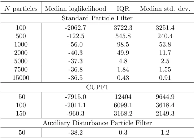
100 -2062.7 3722.3 3251.4 500 -122.5 545.8 240.4 1000 -56.0 98.5 53.8 2000 -40.3 49.9 11.7 5000 -37.3 4.8 2.5 7500 -36.8 1.84 1.55 15000 -36.5 0.43 0.91

CUPF1

50 -7915.0 12404 9644.9 100 -2011.1 6099.1 3618.4 150 -960.3 3168.2 2149.3

Auxiliary Disturbance Particle Filter

50 -38.2 0.3 1.2

Table 2: Quadratic AR(1) model. High nonlinearity, high signal to noise ratio.

N particles Loglikelihood variance Loglikelihood bias Standard Particle Filter

100 0.3824 (.3816,.3837) -0.190 500 0.0809 (0.0807,0.0812) -0.028 1000 0.0403 (0.0402,0.0404) -0.001 2000 0.0211 (0.0211,0.0212) -0.006 5000 0.0081 (0.00808,0.00813) 0.010 7500 0.0052 (0.00519,0.00522) 0.007 15000 0.0027 (0.00269,0.00271) 0.010

CUPF1

50 0.8731 (0.8712,0.8761) -0.416 100 0.3639 (0.3631,0.3652) -0.196 150 0.2869 (0.2863,0.2879) -0.121

Auxiliary Disturbance Particle Filter 50 0.1076 (0.1074,0.1080) -0.117

N particles Loglikelihood variance Loglikelihood bias Standard Particle Filter

100 14.99 (14.96,15.04) -2.90 500 0.8199 (0.8181,0.8228) -0.30 1000 0.3026 (0.3020,0.3037) -0.13 2000 0.1478 (0.1475,0.1483) -0.05 5000 0.0554 (0.0553,0.0556) -0.001 7500 0.0354 (0.0353,0.0355) -0.008 15000 0.0168 (0.0168,0.0169) 0.006

CUPF1

50 43.4 (43.3,43.6) -6.50

100 16.6 (16.6,16.7) -3.06

150 8.17 (8.16,8.20) -1.66

Auxiliary Disturbance Particle Filter 50 0.623 (0.622,0.626) -0.57

N particles Loglikelihood variance Loglikelihood bias Standard Particle Filter

100 1.62×107 (1.61×107,1.63×107) -4396.2

500 7.19×105 (7.17×105,7.21×105) -568.6

1000 1.12×105 (1.116×105_,1.122×105_{) -198.6}

2000 1.083×104 (1.081×104,1.087×104) -53.6 5000 470.3 (469.2,471.9) -9.1

7500 81.8 (81.7,82.1) -3.8

15000 5.33 (5.32,5.35) -1.0 CUPF1

50 3.94×107 (3.93×107,3.96×107) -8611.5

100 1.762×107 (1.758×107_,1.768×107_{) -4538.7}

150 9.30×106 (9.28×106,9.33×106) -2972.2

Auxiliary Disturbance Particle Filter

50 0.2607 (0.2601,0.2616) -0.05

N particles Loglikelihood variance Loglikelihood bias Standard Particle Filter

100 1.057×107 (1.055×107,1.061×107) -3129.4 500 5.781×104 (5.768×104_,5.801×104_{) -156.4}

1000 2897.9 (2891.7,2908.0) -37.5 2000 135.7 (135.4,136.2) -7.8

5000 6.09 (6.07,6.11) -1.27

7500 2.394 (2.389,2.402) -0.57 15000 0.821 (0.820,0.824) -0.10

CUPF1

50 9.30×107 (9.28×107_,9.33×107_{) -1.10×10}4

100 1.309×107 (1.306×107,1.314×107) -3194.6

150 4.62×106 (4.61×106,4.64×106) -1653.8

Auxiliary Disturbance Particle Filter

50 1.522 (1.519,1.527) -1.90

Table 6: Quadratic AR(1) model. High nonlinearity, high signal to noise ratio. 95% confidence intervals for the estimated vari-ances are in brackets.

Parameter Distribution Mean Std. dev.

ρ Beta 0.8 0.1

α Beta 0.333 0.015

δ (%) Gamma 0.5 0.07

σ Gamma 0.01 0.01

N particles Acceptance rate Inefficiencies

α δ ρ σ

Standard Particle Filter

500 2.1 769.7 580.4 491.2 404.1 1500 12.3 43.4 87.0 52.7 56.2 5000 21.8 18.3 19.5 20.4 18.7 10000 24.9 16.8 14.5 18.0 16.5

Auxiliary Disturbance Particle Filter

30 15.2 41.1 27.5 31.2 31.8 50 19.1 25.0 22.1 21.3 23.4 75 21.0 23.3 20.3 20.5 20.4 100 23.3 18.0 17.5 16.4 16.7 150 24.6 22.5 16.1 17.5 18.8 200 25.1 19.2 16.0 17.0 16.8 300 25.9 15.7 13.5 14.5 16.9

N particles Loglikelihood variance Computing time / 10e5

α δ ρ σ

Standard Particle Filter

500 24.03 192.4 145.1 122.8 101.0 1500 2.03 32.5 65.3 39.5 42.2 5000 0.68 45.8 48.7 51.1 46.7 10000 0.28 84.0 72.3 90.2 82.3

Auxiliary Disturbance Particle Filter

30 1.72 9.9 6.6 7.5 7.6 50 1.06 10.0 8.8 8.5 9.4 75 0.67 14.0 12.2 12.3 12.2 100 0.39 14.4 14.0 13.1 13.4 150 0.43 27.0 19.3 21.0 22.6 200 0.25 30.8 25.6 27.1 26.9 300 0.15 37.6 32.5 34.8 40.5

Table 9: Loglikelihood variances and computing times for the neo-classical growth model. The variances of the loglikelihoods are calcu-lated at the true parameter values, α = 1/3, ρ = 0.8, δ = 0.05 and

σ2 = 0.022. The value of k = 16 is used in calculating computing times.

Parameter Distribution Mean Std. dev.

γ Gamma 2 0.5

g (%) Gamma 1.9 0.15

rf (%) Normal 1.0 0.01

φ Beta 0.8 0.1

σν (%) Gamma 0.8 0.03

ση (%) Gamma 0.1 0.03

σ (%) Gamma 5 0.7

Table 10: Priors for the structural parameters in the asset pric-ing model. Values for g and rf and their standard deviations are in annualised percentage terms. The prior distribution of

N particles Posterior Mean (Std. Dev. in brackets)

g (%) γ φ rf (%) σ (%) ση (%) σν (%)

Standard Particle Filter

200 2.9 (0.28) 0.93 (0.356) 0.97 (0.007) 1.0 (0.01) 7.4 (0.43) 0.8 (0.07) 0.8 (0.05) 500 2.8 (0.20) 0.87 (0.334) 0.97 (0.008) 1.0 (0.01) 7.5 (0.50) 0.8 (0.06) 0.8 (0.04) 1000 2.9 (0.22) 0.94 (0.399) 0.97 (0.009) 1.0 (0.01) 7.3 (0.48) 0.8 (0.08) 0.8 (0.03)

Auxiliary Disturbance Particle Filter

30 2.9 (0.19) 0.86 (0.309) 0.97 (0.007) 1.0 (0.01) 7.4 (0.46) 0.8 (0.06) 0.8 (0.02) 50 2.8 (0.21) 0.85 (0.309) 0.97 (0.008) 1.0 (0.01) 7.4 (0.43) 0.8 (0.06) 0.8 (0.03)

Table 11: Parameter estimates for the asset pricing model with standard errors in brackets. Values for

g andrf and their standard deviations are in annualised percentage terms.

N particles Acc. rate Inefficiencies

g γ φ rf σ ση σν

Standard Particle Filter

200 5.0 115.8 195.9 444.5 129.0 477.6 359.9 128.7 500 11.4 59.7 63.1 58.7 63.1 48.9 52.9 34.3 1000 13.9 39.6 42.7 48.3 42.6 57.8 30.5 55.5

Auxiliary Disturbance Particle Filter

30 11.4 52.2 38.0 50.0 112.5 49.3 51.9 54.9 50 14.1 36.5 85.0 98.7 58.2 48.4 35.7 47.9

Table 12: MCMC parameter inefficiencies for the asset pricing model.

N particles Computing Times

g γ φ rf σ ση σν

Standard Particle Filter

200 57.4 97.2 220.5 64.0 236.9 178.5 63.8 500 74.0 78.2 72.8 78.2 60.6 65.6 42.5 1000 98.3 105.8 119.8 105.6 143.2 75.6 137.7

Auxiliary Disturbance Particle Filter

30 27.6 20.1 26.4 59.4 26.0 27.4 29.0 50 32.1 74.8 86.9 51.3 42.6 31.4 42.2