The environmental Kuznets curve, economic growth, renewable and non renewable energy, and trade in Tunisia

Munich Personal RePEc Archive

The environmental Kuznets curve,

economic growth, renewable and

non-renewable energy, and trade in

Tunisia

Ben Jebli, Mehdi and Ben Youssef, Slim

Jendouba University, Manouba University

10 December 2013

Online at

https://mpra.ub.uni-muenchen.de/52127/

The environmental Kuznets curve, economic growth, renewable and

non-renewable energy, and trade in Tunisia

Mehdi Ben Jebli

LAREQUAD & FSEGT, University of Tunis El Manar, Tunisia University of Jendouba, ISI du Kef, Tunisia

benjebli.mehdi@gmail.com

Slim Ben Youssef∗∗∗∗

LAREQUAD & FSEGT, University of Tunis El Manar, Tunisia Manouba University, ESC de Tunis, Tunisia

slim.benyoussef@gnet.tn

First Version: December, 2013

Abstract: We use the autoregressive distributed lag (ARDL) bounds approach to cointegration in order to investigate the short and long-run relationship between per capita

CO2 emission, GDP, renewable and non-renewable energy consumption and trade openness

for Tunisia during the period 1980-2009. The Fisher-statistic for cointegration is established

when CO2 emission is defined as a dependent variable. The stability of coefficients in the long

and short-run is examined. Short-run Granger causality suggests that there is a one way causality relationship from economic growth and trade openness (exports and imports) to emissions, whereas there is no causality running from renewable and non-renewable energy consumption to emissions. The results from the long-run relationship suggest that

non-renewable energy consumption contributes positively in explaining CO2 emission (for both

models), whereas renewable energy affects CO2 emission negatively (for the model with

exports). The contribution of trade openness is positive and statistically significant in the long-run. The Environmental Kuznets Curve (EKC) that assumes an inverted U-shaped

relationship between per capita CO2 emissions and output is not supported in the long-run.

This means that Tunisia has not yet reached the required level of per capita GDP to get an inverted U-shaped EKC.

Keywords: Environmental Kuznets Curve; Renewable and non-renewable energy; Trade openness; Autoregressive distributed lag; Tunisia.

JEL Classification: C22, F14, Q42, Q43, Q54

1. Introduction

To our knowledge, there is no cross-sectional study that has addressed the causal relationship between environmental pollution, renewable and non-renewable energy consumption, and trade openness. This study tries to test the validity of the so-called Environmental Kuznets Curve (EKC) hypothesis for the case of Tunisia. We will evaluate the impact of per capita real GDP, per capita renewable and non-renewable energy consumption,

and per capita trade openness on per capita CO2 emission in Tunisia.

Several econometric studies focuses on the dynamic linkages between emissions of CO2,

energy consumption and economic growth (e.g. Ang 2007, 2008; Ozturk and Acaravci 2010;

Soytas et al. 2007). Other recent papers reveal that trade openness is one of the most

important factors that may affect pollution emissions in the short and long-run links through the energy used for production. However, they incorporate trade openness (exports plus

imports) in the environmental specification model (e.g. Halicioglu 2009; Jayanthakumaran et

al. 2012). Our paper differs from the existing literature by the fact that we try to examine how

renewable and non-renewable energy consumption and trade can affect polluting emissions. In fact, we use the same approach employed in the previous studies with a multivariate framework. However, in our study we separate energy in per capita renewable and non-renewable energy. The trade openness is considered as a supplementary variable to the dynamic nexus.

In order to protect the environment and to save the Earth’s biosphere from pollution, it’s

necessary to reduce CO2 emissions to prevent predictable disasters. According to the World

Bank (2011), Tunisia recorded an annual average of 11403.5 tons metrics for the whole period 1960-2008. The highest level of emissions is 25012.6 tons metrics in 2008 and the lowest level is 1727.2 tons metrics in 1960. Some recent empirical papers study the causal

relationship between CO2 emissions, energy consumption and economic growth for the

Tunisian case. Fodha and Zaghdoud (2010) study the causal links between environmental

indicators (CO2, SO2) and economic growth for Tunisia, using cointegration analysis. They

come to the conclusion that more investment in pollution abatement expense and more severe emissions reduction policies will not hurt economic growth. Chebbi (2010) debates the long

and short-run causal links between energy consumption, economic growth and CO2 emissions

for Tunisia over the period 1975-2005. The author concludes that prudent energy and environmental policies should distinguish the differences in the relationship between energy

consumption and output growth by sector. Chebbi et al. (2011) use cointegration techniques

to examine the causality between trade openness, economic growth and CO2 emissions for

Tunisia. They recommend that the direct effect of trade openness is positive on emissions both in the short and the long-run but the indirect effect is negative.

2. Literature review

There are several empirical studies that are completely devoted to test the validity of the EKC hypothesis for a single country and/or a balanced panel. These studies can be classified in two categories of empirical research. The first category is supposed to examine the dynamic relationship between economic growth and environmental pollutants (e.g.

Akbostanci et al. 2009; Fodha and Zaghdoud 2010) or between economic growth, energy

consumption and environmental pollutants (e.g. Ang 2007, Arouri et al. 2012). The second

category is supposed to examine the dynamic relationship between economic growth, energy consumption, environmental pollutants and trade (e.g. Suri and Chapman 1998; Halicioglu

2009; Jayanthakumaran et al. 2012).

Concerning the first kind of literature, Ang (2007) studies the case of France over the annual period 1960-2000 by using cointegration and vector error-correction modeling techniques and his results provide the existence of a robust run relationship. The long-run relationship supports that economic growth exerts a causal influence on the growth of energy consumption and the growth of pollution. The results also provide that in the short-run there is a unidirectional causality running from growth of energy consumption to economic

growth. Arouri et al. (2012) employ cointegration techniques to examine the relationship

long-run, energy consumption has a positive significant impact on CO2 emissions. Also real

GDP exhibits a quadratic relationship with CO2 emissions for the region as a whole. The

long-run elasticities of income and its square satisfy the EKC hypothesis in most studied countries. Emission reductions have been realized in the MENA region, even though the

region exhibited economic growth over the period 1981–2005. In the case of Tunisia, Fodha

and Zaghdoud (2010) investigate the relationship between economic growth and pollutant

emissions (CO2 and SO2) over the annual period 1961-2004. They find that there is a long-run

cointegration relationship between emissions of the two pollutants and GDP. They also conclude that an emission reduction policy and more investment in pollution abatement will

not reducethe Tunisian’s economic growth.

Concerning the second kind of literature, Halicioglu (2009) examine the causal relationship between carbon emissions, energy consumption, income, and trade in the case of Turkey by using the autoregressive distributed lag (ARDL) bounds testing to cointegration procedure. The results from the bounds indicate that there are two forms of long-run equilibrium. The first form is that carbon emissions are explained by energy consumption, income and trade, and the second form is that carbon emissions, energy consumption, and trade are determinants of income. From the first form which respects the EKC hypothesis, the empirical results suggest that income is the most significant variable followed by energy consumption and trade.

Our study differs from the existing literature by the fact that we try to test how economic growth, renewable and non-renewable energy consumption, and trade openness can affect pollutant emissions for the case of Tunisia. Practically, our model follows the same

econometric specification developed by Halicioglu (2009) and Jayanthakumaran et al. (2012)

with the difference that, in our model, trade openness distinguishes between real exports and real imports. By separating these two trade variables, we can know which of these variables

contributes to CO2 emissions, when renewable energy consumption is used for economic

production.

The objectives of our empirical estimations are to investigate the dynamic causal relationship between variables and to examine how these variables are associated with the long-run equilibrium. In particular, the aim of this study is to test whether the environmental

Kuznets curve relationship between per capita CO2 emissions, real GDP, renewable and

non-renewable energy consumption and trade openness grips in the long-run or not. As mentioned in the previous studies, empirical specification includes foreign trade to reduce omitted variable bias (Jalil and Mahmud 2009). However, in our model we decompose the impact of trade openness in real exports and real imports in order to clarify which variable may affects environmental conditions. Thus, our empirical analysis uses ARDL techniques to check for long-run association between variables using two specification models: one with exports and

one with imports. Our statistical analysis follows five steps: i) examines the stationary

proprieties, ii) selects the optimal lag length order of the vector autoregressive (VAR) model,

iii) tests the existence of the long-run relationship among variables through Wald test based

on Fisher statistic, iv) establishes the direction causality between variables by using pairwise

Granger causality tests, v) estimates the short and long-run parameters, and vi) tests the

stability of the model.

3. Data and methodology

3.1. Data and specification model

The aim of this study is to investigate the causal linkages between environmental indicator

and trade openness (O) for the case of Tunisia. Following the methodology developed by Ang

(2007), Holicioglu (2009) and Jayanthakumaran et al. (2012) into a single multivariate

framework, we develop a model based on the EKC hypothesis:

2

( , , , , )

t t t t t t

E = f Y Y RE NRE O (1)

With respect to this methodology, the log linear quadratic EKC equation which is specified to examine the long-run relationship between these variables is given as follow:

2

0 1. 2. 3. 4. 5.

t t t t t t t

e =α α+ y +α y +α re +α nre +α o +ε (2)

where t, α₀, andεdenote the time, the fixed country effect and the white noise stochastic

disturbance term, respectively. The environmental indicator (e) is defined as the CO2

emissions measured in metric tons per capita, output (y) indicates real GDP per capita

measured in constant 2005 US dollars, (y2) is the square of real GDP per capita, (re) indicates

renewable energy consumption per capita defined as geothermal, solar, wind, tide and wave, biomass and waste, and hydroelectric power consumption measured in billion kilowatt hours.

(nre) indicates non-renewable energy consumption per capita defined as the sum of oil,

natural gas and coal measured in billion kilowatt hours. Data series on renewable and non-renewable energy consumption are divided by population number to get the per capita unit.

Trade openness variable (o)1 is defined as per capita real merchandise exports (ex) in US

dollars or per capita real merchandise imports (im) in US dollars. These variables are

transformed from the current value to the real one by dividing them by the consumer price index (pc), and then they are divided by the population number to get the per capita unit. The database is selected to get the maximum number of observations depending on the availability

of data. Data on real GDP per capita, CO2 emissions per capita, population, merchandise

exports and merchandise imports from 1980 to 2009 are obtained from the World Bank (2013). Renewable and non-renewable energy data are obtained from the U.S. Energy Information Administration (2012) online database. Data on (pc) are obtained from the Penn

World Table version 7.1 (Heston et al. 2012). All variables presented in Eq. (2) are in natural

logarithms.

The coefficients α_{i i(=1,2,3,4,5)} are the long-run elasticities corresponding to each explanatory

variable. With respect to the EKC hypothesis, the sign of α₁ is expected to be positive (

1 0

α > ), whereas α₂ is expected to be negative (α₂<0). Indeed, an increase in real GDP

would lead to an increase in emissions, whereas an increase in the square of real GDP would

lead to a decrease in emissions. The expected sign of α₃ is negative because an increase in

per capita renewable energy consumption would decrease per capita emissions. The sign of

4

α is expected to be positive (α₄ >0) given that emissions increase if the consumption of

non-renewable energy is higher. The signs of α₅ is expected to be mixed and depend on the

economic level of the country. Grossman and Krueger (1995), Halicioglu (2009) and Shahbaz

et al. (2012) reveal that the sign of trade openness slope parameter is positive if the dirty

industries of developing economies are producing with heavy share of CO2 emissions.

1

3.2. Unit root tests

To check for integration order of each variable, we use traditional unit root tests. All variables are tested at level and after the first difference using a test of Fisher based on the Augmented Dickey Fuller (1979) (ADF-Fisher) and Phillips and Perron (1988) (P-P Fisher). These two tests assume that the null hypothesis is that there is a unit root, whereas the alternative hypothesis is that variables are stationary after first integration.

3.3. ARDL bounds testing approach

A number of cointegration techniques can be used for testing the existence of a long-run relationship between analysis variables. One of these cointegration techniques named autoregressive-distributed lag (ARDL) or ARDL bounds approach has been employed by Pesaran and Pesaran (1997), Pesaran and Smith (1998), Pesaran and Shin (1999), and Pesaran

et al. (2001). As revealed in previous studies, the ARDL approach used for cointegration has

several econometric advantages:

(i) Compared to other cointegration techniques that require that all variables should

be integrated into the same order, ARDL bounds can be employed without inspecting the integration order of variables. This technique examines the long-run relationship between variables and is appropriate whether regressors are purely integrated of order zero I(0), purely order one I(1) or fractionally integrated (Pesaran and Pesaran 1997).

(ii) The long-run and the short-run informations are integrated in the same

specification derived from ARDL after linear transformation, and are simultaneously estimated which removes the problems associated with serial correlation and endogeneity (Pesaran and Shin, 1999).

(iii) Compared to other cointegration approaches such as Engle and Granger (1987),

Johansen and Juselius (1990), and the fully modified OLS procedures of Phillips and Hansen (1990), the ARDL approach for cointegration recommends better results with a small sample (Haug, 2002).

The ARDL representation of Eq. (2) is formulated as follows:

2

0 1 2 3 4 5

1 1 1 1 1

2

6 7 1 8 1 9 1 10 1 11 1 12 1

1

p p p p p

t i t i i t i i t i i t i i t i

i i i i i

p

i t i t t t t t t t

i

e e y y re nre

o e y y re nre o

θ θ θ θ θ θ

θ θ θ θ θ θ θ π

− − − − − = = = = = − − − − − − − = ∆ = + ∆ + ∆ + ∆ + ∆ + ∆ + ∆ + + + + + + +

∑

∑

∑

∑

∑

∑

Where∆ and π_t are the first difference and the error terms, respectively. According to

Pesaran et al. (2001), the long-run linkage between variables is tested for the joint

significance of estimated coefficients of the lagged level. This test can be done after determining the number of optimal lag length for regression which is selected by the Schwarz Information Criteria (SIC). Based on the Wald tests, the Fisher-statistic is calculated in order

to test the existence of cointegration among the variables. Pesaran et al. (2001) have

developed this recent approach for cointegration which is established on the null hypothesis of

no long-run association between the variables (H₀:θ θ θ θ₇ = = =_{8 9 10} =θ₁₁=θ₁₂ =0), against

the alternative hypothesis of long-run relationship (H₁:θ θ θ θ₇ ≠ ≠_{8 9} ≠ ₁₀ ≠θ₁₁≠θ₁₂ ≠0). The

calculated value is compared with two terminal critical values provided by Pesaran et al.

the lower critical bound value, whereas the second terminal assumes that all variables are I(1) and corresponds to the upper bound value. In this case, three assumptions are possible to interpret Fisher-statistic value: if the computed F-statistic exceeds the upper critical value, then we reject the null hypothesis of no cointegration. If the computed Fisher-statistic falls behind the lower critical value, then we cannot reject the null hypothesis of no cointegration between variables. Finally, if the calculated value falls within lower and upper critical values,

then the result is inconclusive. In this case, Banerjee et al. (1998) suggest that the existence of

cointegration can be tested using the significance of the error correction term. Diagnostic tests are computed to assess the robustness of the empirical model based on the serial correlation, residual heteroskedasticity, and normality tests.

3.4. Granger causality test

After establishing the existence of long-run relationship between variables using ARDL bounds technique, we run the Granger causality test to check for the direction causality between them. Given the existence of long-run association among variables, it is required to

rely on the significance of the error correction term (ECT). However, Engle and Granger

(1987) techniques are employed to examine the short and long-run association among variables in two steps. Firstly, we estimate the long-run coefficients of Eq. (2) in order to obtain the residuals. Secondly, we estimate the coefficients related to the short-run adjustment. The error correction model of the long-run equation is given as follows:

2

0 1 2 3 4 6 7

1 1 1 1 1 1

1

p p p p p p

t i t i i t i i t i i t i i t i i t i

i i i i i i

t t

e e y y re nre o

ECT

λ λ λ λ λ λ λ

α η

− − − − − −

= = = = = =

−

∆ = + ∆ + ∆ + ∆ + ∆ + ∆ + ∆

+ +

∑

∑

∑

∑

∑

∑

(4)

where ∆ indicates the first difference, η_t denotes the standard error term, ECTt-1 is the lagged

error term generated from Eq. (4), and α indicates the speed of adjustment coefficients. The

Granger causality tests are employed to investigate the long-run relationship with the negative

sign of the lagged ECT and its statistical significance using t-statistic, and the short-run

relationship by lagged differences of variables specified in each equation using F-statistic.

3.5. Model stability tests

To assess the stability of the long and short-run coefficients of the empirical model, we apply the cumulative sum (CUSUM) and the cumulative sum of the square (CUSUMSQ) methods of Brown et al. (1975). These tests are presented graphically and based on the ECM of Eq. (3). Halicioglu (2009) shows that the existence of a long-run association between variables does not mean that the estimated coefficients are stable. He also shows that the tests

of Brown et al. (1975) are more powerful than other kinds of stability tests such as Hansen

(1992) and Hansen and Johansen (1993) because these latter require that variables are integrated of order one and also does not incorporate short-run estimated coefficients of the model.

4. Empirical analysis

ADF and P-P Fisher tests to check for the integration order. The null hypothesis is that the series has a unit root, whereas alternative hypothesis is that the series is stationary. Unit root tests are done in the cases of intercept, and intercept and trend.

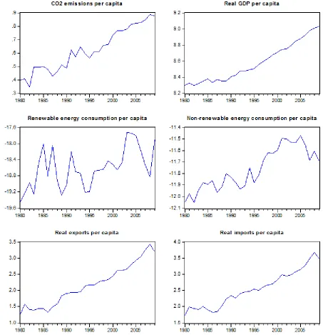
Fig 1. Natural logarithms of analysis variables

Fig 1 reports the time series plots in natural logarithms variations of per capita CO2

Table 1. Unit root tests

Variables ADF test statistic P-P test statistic

levels k 1st differences k levels k 1st differences k

e -0.632274 0 -8.229403a 0 -0.155010 5 -13.44154a 8

y 1.977996 0 -5.210576a 0 3.111978 5 -5.218914a 2

Intercept y2 2.153832 0 -5.048737a 0 3.351556 5 -5.090662a 3

re -3.104125 0 -6.194616a 0 -3.009169 3 -12.45968a 18

nre -1.720357 0 -6.139479a 0 -1.686509 1 -6.296108a 2

ex -0.108966 0 -5.451014a 0 0.189785 5 -5.469238a 1

im -0.102314 0 -4.219926a 1 0.173534 5 -4.483382a 5

e -4.021792 0 -4.707682a 6 -4.000112 1 -14.35166a 9

y -3.424231 6 -6.860267a 0 -1.521709 5 -8.904239a 12

Intercept y2 -3.284282 6 -6.854059a 0 -1.428623 6 -9.734739a 14

and trend re -3.336945 1 -5.081314a 4 -3.494058 5 -10.94124a 19

nre -2.124582 0 -5.300432a 1 -2.036576 2 -6.396545a 3

ex -2.577508 0 -5.750590a 0 -2.463142 3 -5.868984a 5

im -3.567522 1 -4.719817a 0 -2.347848 3 -4.987980a 10

Note:ADF and P-P denote augmented Dickey-Fuller and Phillips-Perron, respectively. k is the lag length that is determined automatically and based on the Schwarz Information Criterion (SIC). a, denotes statistical significance level at the 1%.

Table 1 reports the results of the ADF and P-P unit root tests. The result from ADF

statistic test shows that per capita CO2 emissions, real GDP per capita, square of real GDP per

capita, renewable and non-renewable energy consumption per capita, real exports per capita, and real imports per capita are non-stationary at level, whereas after first difference they become stationary at the 1% significance level. Thus, the ADF test confirms that all series are I(1). From P-P unit root test, the results show the same outcomes and confirm the stationary proprieties of ADF test. Finally, these two tests ensure that none of the variables is integrated

with an upper order 1 and approve that all series are integrated of order one, I(1)2.

As previously shown, the ARDL bounds procedure allows that analysis series must be integrated in order of zero or in order of one. However, the integration test results reveal that all variables are stationary after first difference. Two steps have been recommended for the ARDL cointegration test. The first step consists in checking for the optimal number of lags for the vector autoregressive (VAR) model. Thereby, the number of lags on the first difference of variables is obtained via the unrestricted VAR by means of Log likelihood (LogL), Log likelihood ratio (LR), final prediction error (FPE), Akaike information criterion (AIC), Schwarz information criterion (SIC), and Hannan-Quinn information criterion (HQ) which are employed to determinate the optimal number of lags.

For the model with exports (resp. imports) the lag selection criteria results for VAR models are established. With two as a maximum number of lags, the estimated results of most criteria suggest that the optimal number of lags is equal to two (VAR (p=2)), and SIC suggests a maximum lag of one (VAR (p=1)). However, with a number of lag 2, the adjustment to the long-run equilibrium is not proved, whereas with a number of lag 1 the

adjustment is significant.3 In the light of these statistics, we decide to use (VAR (p=1)).

2

The use of the ARDL bounds technique cannot be used if one or more time series are integrated of order two or beyond. However, testing for cointegration assumes that all series are whether I(0) or I(1) or fractionally integrated in order to avoid spurious results (Ouattara 2004, Jalil and Mahmud 2009).

3

The second step of the ARDL bounds approach consists in the estimation of Eq. (3) using OLS estimation method and the Wald test (Fisher-statistic) for the joint significance of the long-run coefficients of lagged levels of variables in order to test the existence of the long-run association using bounds test (coitegration test). This study employs the critical values of

Pesaran et al. (2001) for the F-test to check for cointegration. For the choice of lag length, we

use AIC and SIC criteria. A maximum of three lags is appropriate for our test.

Table 2. F-test for cointegration: model with exports

Critical bounds of the F-statistica _10%

e=f(y,y2,re,nre,ex) Lower bounds I(0) Upper bounds I(1)

2.262 3.367

F-statistics model with exports 206.275*

Notes: * indicates statistical significance at the 10 % level. a indicates critical values at the 10 % level. 2.262 is the critical value for the lower bounds and 3.367 is the critical value for the upper bounds. Critical values are provided by Pesaran et al. (2001) for the case II (with intercept and no trend).

For the model with exports, the computed value of the Fisher-statistic is equal to 206.275. This value is higher than the lower and the upper bounds values (see Table 2). This result confirms that there is a long-run relationship (cointegration) among variables when the

emissions of CO2 are defined as a dependent variable. According to the AIC and SIC lag

specification for emissions, the result reveals an ARDL (3, 3, 3, 3, 3, 3) for the model with exports.

Table 3. F-test for cointegration: model with imports

Critical bounds of the F-statistica _1%

e=f(y,y2,re,nre,im) Lower bounds I(0) Upper bounds I(1)

4.011 5.331

F-statistics model with imports 29.512*

Notes: * indicates statistical significance at the 1 % level. a indicates critical values at the 1 % level. 4.011 is the critical value for the lower bounds and 5.331 is the critical value for the upper bounds. Critical values are provided by Pesaran et al. (2001) for the case III (with intercept and trend).

For the model with imports, the computed value of the Fisher-statistic is equal to 29.512. This value is higher than the lower and the upper bounds values (see Table 3). This result confirms that there is a long-run relationship (cointegration) among variables when the

emissions of CO2 are defined as a dependent variable. Based on the AIC and SIC lag

Table 4. Granger causality tests (model with exports)

Variable

Short-run Long-run

e y y2 re nre ex ECT

e - 11.5977 (0.0022)*** 10.9076 (0.0028)*** 0.07934 (0.7804) 0.53993 (0.4690) 9.00307 (0.0059)*** -0.245502 [-2.56104]**

y 2.50563

(0.1255) -

0.63570 (0.4325) 0.82962 (0.3707) 1.49591 (0.2323) 1.47237 (0.2359) -3.265472 [-2.30455]

y2 2.45813

(0.1290)

0.67732

(0.4180) -

0.72562 (0.4021) 1.54532 (0.2249) 1.49294 (0.2327) 3.172411 [2.32219]

re 4.45976

(0.0445)**

3.71442 (0.0649)*

3.71566

(0.0649)* -

8.72536 (0.0066)*** 2.99431 (0.0954)* -0.337112 [-4.19423]***

nre 1.05278

(0.3143) 0.98038 (0.3312) 0.88758 (0.3548) 0.43092

(0.5173) -

0.30592 (0.5849)

-0.326662 [-1.84811]*

ex 1.42402

(0.2435) 2.64627 (0.1159) 2.48735 (0.1269) 0.37026 (0.5481) 0.57033

(0.4569) -

-0.137690 [-1.48903]

Notes: ***, **, * indicate statistical significance at the 1%, 5% and 10% levels, respectively. P-values are presented in parentheses and t-statistics are in brackets.

For the model with exports, the results from the short and long-run Granger causality tests are reported in Table 4. The Short-run dynamics results reveal that there is evidence of a

unidirectional causality from real GDP per capita to CO2 emissions per capita and from the

square of real GDP per capita to CO2 emissions per capita at the 1% significance level,

whereas there is no causal links that run from energy consumption per capita (renewable and

non-renewable) to CO2 emissions per capita. The interconnection between real GDP per

capita (or the square of real GDP per capita) and renewable energy consumption per capita is unidirectional. Indeed, there is a one way causal relationship without feedback that runs from real GDP per capita (the square of real GDP per capita) to renewable energy consumption, but there are no links between real GDP per capita (or the square of real GDP per capita) and non-renewable energy per capita. The short-run results show also that there is evidence of a

unidirectional causality from real exports per capita to CO2 emissions per capita and to

renewable energy per capita. Also, there is a unidirectional causality running from per capita

CO2 emissions and per capita non-renewable energy consumption to renewable energy

consumption.

The long-run dynamics results reveal that, for the model with exports, the error correction

terms coefficients of CO2 emissions per capita, renewable and non-renewable energy

consumption per capita are negative and statistically significant at the 5%, 1% and 10%

significance levels, respectively. It means that there is a long-run association running: i) from

real GDP per capita, square of real GDP per capita, renewable and non-renewable energy

consumption per capita and real exports per capita to CO2 emissions per capita, ii) from CO2

emissions per capita, real GDP per capita, square of real GDP per capita, non-renewable energy consumption per capita and real exports per capita to renewable energy consumption

per capita, and iii) from CO2 emissions per capita, real GDP per capita, square of real GDP

Table 5. Granger causality tests (model with imports)

Variable

Short-run Long-run

e y y2 re nre im ECT

e - 11.5977 (0.0022)*** 10.9076 (0.0028)*** 0.07934 (0.7804) 0.53993 (0.4690) 14.1019 (0.0009)*** -0.504980 [-2.39564]**

y 2.50563

(0.1255) -

0.63570 (0.4325) 0.82962 (0.3707) 1.49591 (0.2323) 1.71039 (0.2024) -2.615209 [-1.72953]

y2 2.45813

(0.1290)

0.67732

(0.4180) -

0.72562 (0.4021) 1.54532 (0.2249) 1.68288 (0.2059) 2.519834 [1.75939]

re 4.45976

(0.0445)**

3.71442 (0.0649)*

3.71566

(0.0649)* -

8.72536 (0.0066)*** 3.56904 (0.0701)* 0.181750 [2.39568]

nre 1.05278

(0.3143) 0.98038 (0.3312) 0.88758 (0.3548) 0.43092

(0.5173) -

0.54270 (0.4679)

-0.411122 [-2.01252]**

im 1.48440

(0.2340) 4.00694 (0.0559)* 3.84175 (0.0608)* 0.78193 (0.3847) 0.27521

(0.6043) -

-0.162334 [-0.82061]

Notes: ***, **, * indicate statistical significance at the 1%, 5% and 10% levels, respectively. P-values are presented in parentheses and t-statistics are in brackets.

For the model with imports, the results from the short and the long-run Granger causality tests are reported in Table 5. In the short-run, there is a unidirectional causality

without feedback from real GDP per capita (or the square of real GDP per capita) to CO2

emissions per capita. However, there are no causal links running from energy consumption

per capita (renewable and non-renewable) to CO2 emissions per capita. There is also a one

way causal relationship running from real GDP per capita (or the square of real GDP per capita) to renewable energy consumption per capita, but there is no causality between non-renewable energy per capita and real GDP per capita. Granger causality results suggest that

there is a one way causality running from real imports per capita to CO2 emissions per capita

at the 1% significance level. There is also a short-run causality running from CO2 emissions

per capita, non-renewable energy consumption per capita and real imports per capita to renewable energy consumption per capita. Finally, we find that there is a short-run unidirectional causality that runs from real GDP per capita (square of real GDP per capita) to real imports per capita at 10% significance level.

The long-run dynamics results reveal that, for the model with imports, the error

correction terms coefficients of CO2 emissions per capita and non-renewable energy

consumption per capita are both negative and statistically significant at the 5% level. It means

that there is a long-run association running: i) from real GDP per capita, square of real GDP

per capita, renewable and non-renewable energy consumption per capita and real imports per

capita to CO2 emissions per capita, and iii) from CO2 emissions per capita, real GDP per

Fig.2 Pairwise Granger Causality results

The most interesting reading that can be drawn from the short-run causality recommends that there are direct and indirect interdependencies between our main variables. According to Fig 2, the short-run causality between emissions, economic growth, renewable and non-renewable energy consumption and trade openness (real exports and real imports) can be classified in two groups of causality relationship. The first group includes variables that affect emissions which are economic growth and trade openness, and the second group includes the explanatory variables that may affect directly renewable energy consumption in the short-run.

Regarding the dependence between emissions and economic growth, our finding suggests a one way causality running from economic growth to emissions. This result is consistent with the findings of Haggar (2012) for the case of Canadian industrial sector and

Jalil and Mahmud (2009) for China. The presence of a unidirectional causality relationship

from economic growth to emissions recommends that any fluctuations in economic growth may change the environmental degradations but any effort that may reduce emissions will not affect economic growth. There is also a unidirectional causality running from exports and imports to emissions. This result means that trade openness policy has a vital role in explaining emissions. This result is not on line with the finding of Halicioglu (2009) for Turkey.

The second group of short-run causality includes the explanatory variables that may affect directly renewable energy consumption. Interestingly, pairwise Granger causality affirms that emissions, economic growth, non-renewable energy consumption and trade have a significant impact on renewable energy consumption. The causality relationship that runs from emissions to renewable energy consumption is consistent with the findings of Menyah

and Wolde-Rufael (2010) for the US and Apergis et al. (2010). Contrary to the result of

Apergis and Payne (2010a) for a panel of OECD countries, Apergis and Payne (2010b) for a panel of Eurasia countries, Apergis and Payne (2011) in Central America, and Apergis and Payne (2012) for a panel of 80 countries who find a bidirectional causality between economic growth and renewable energy consumption, our results reveal a unidirectional causality from economic growth to renewable energy consumption which are on line with Menyah and Wolde-Rufael (2010). The short-run causality also reveals the existence of a unidirectional causality from non-renewable energy consumption to renewable energy consumption. This

Non-renewable energy Renewable

energy

Real imports Real exports

result is contrary to the finding of Apergis and Payne (2012) who suggest the existence of a bidirectional causality. The presence of a unidirectional causality from trade openness to renewable energy consumption implies that more trade has an influence on the use of

renewable energy. This finding is not similar to the result of Ben Aissa et al. (2013) for a

panel of 11 African countries. Indeed, these authors conclude that there is no evidence of causality between renewable energy consumption trade openness in both the short and long-run relationship.

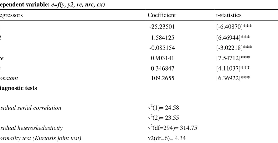
Table 6. Long-run estimates: ARDL model (model with exports)

Dependent variable: e=f(y, y2, re, nre, ex)

Regressors Coefficient t-statistics

y -25.23501 [-6.40870]***

y2 1.584125 [6.46944]***

re -0.085154 [-3.02218]***

nre 0.903141 [7.54712]***

ex 0.346847 [4.11037]***

Constant 109.2655 [6.36922]***

Diagnostic tests

residual serial correlation γ2(1)= 24.58

γ2(2)= 23.55

residual heteroskedasticity γ2(df=294)= 314.75

Normality test (Kurtosis joint test) γ2(df=6)= 4.34

Notes: *** indicates statistical significance at the 1% level. Diagnostic test for residual is based on the serial correlation test and normality test. γ2(1)=24.58 and γ2(2)=23.55 are the Lagrange multiplier test statistics for the first and the second serial correlation, respectively.

γ2(df=294)= 314.75is the joint statistic value of the residual heteroskedasticity and γ2(df=6)=4.34 indicates the joint statistic of normality test based on Cholesky for orthogonalization method.

For the model with exports, the estimated long-run coefficients results are reported in Table 6. All estimated coefficients are statistically significant at the 1% level, and the majority are positive exception the coefficients of per capita real GDP and renewable energy consumption which are negative. A 1% increase in per capita real GDP will decrease the per

capita emissions of CO2 by 25.23%, and a 1% increase in per capita the square of real GDP

leads to an increase of per capita emissions by 1.58%. This result does not support the EKC hypothesis which affirms that, when the per capita real GDP is not sufficiently high, the per

capita emissions of CO2 increase with the per capita real GDP at a high rate, and then, when

the per capita real GDP is sufficiently high, the per capita emissions of CO2 increase with the

per capita real GDP at a lower rate. A 1% increase in the consumption of renewable energy leads to a decrease in emissions by 0.08%, a 1% increase in the consumption of non-renewable energy will increase emissions by 0.90%, and a 1% increase in real exports will increase emissions by 0.35%. Thus, in the long-run, more renewable energy use contribute to

reduce slightly CO2 emissions because in Tunisia the proportion of per capita renewable

energy consumed with respected to the per capita total energy consumption is very week

Table 7.Long-run estimates: ARDL model (model with imports)

Dependent variable: e=f(y, y2, re, nre, im)

Regressors Coefficient t-statistics

y -12.33947 [-4.41097]***

y2 0.762715 [4.39614]***

re 0.032472 [1.44816]

nre 0.511276 [5.90800]***

im 0.374455 [5.08595]***

Constant 56.07751 [3.73710]***

Diagnostic tests

residual serial correlation γ2(1)= 56.55

γ2(2)= 42.78

residual heteroskedasticity γ2(df=294)= 321.92

Normality test (Kurtosis joint test) γ2(df=6)= 5.35

Notes: *** indicate statistical significance at the 1% level. Diagnostic test for residual is based on the serial correlation test and normality test. γ2(1)=56.55 and γ2(2)=42.78 are the Lagrange multiplier test statistics for the first and the second serial correlation, respectively.

γ2(df=294)= 321.92is the joint statistic value of the residual heteroskedasticity and γ2(df=6)=5.35 indicates the joint statistic of normality test based on Cholesky for orthogonalization method.

The results of the long-run estimates of the model with imports are reported in Table 7. All coefficients are statistically significant at the 1% level exception for renewable energy consumption coefficient which is not statistically significant. The estimated coefficient of per capita real GDP is negative and the estimated coefficient of per capita the square of real GDP is positive, implying that the EKC hypothesis is not verified. Indeed, a 1% increase in per capita real GDP decreases per capita emissions by 12.34% and a 1% increase in per capita the square of real GDP increases per capita emissions by 0.76%. A 1% increase in per capita non-renewable energy consumption increases emissions by 0.51%, and a 1% increase in per capita real imports increases emissions by 0.37%. The diagnostic test results show that, for the long-run models, there is no serial correlation, no problem of white heteroskedasticity, and the residual is normally distributed.

Table 8.Short-run estimates: ECM-model with exports

Dependent variable: (e)

Regressors Coefficient t-statistics

(y) 19.68467 [1.81118]*

(y2) -1.227012 [-1.75291]*

(re) -0.017279 [-0.84855]

(nre) -0.283980 [-2.42070]**

(ex) -0.288150 [-3.02791]***

Constant 0.037394 [3.01424]***

ECT _{-0.245502 [-2.56104]**}

Diagnostic tests R2=0.57

F-statistic=3.85 prob(F-statistic)=0.008 Normality test= 3.05 (0.5720)

Heteroskedasticity test=1.38 (0.2515)

Serial Correlation LM Test=0.84 (0.4461)

Durbin-Watson= 1.90

Note: *, **, *** indicate statistical significance at the 10%, 5% and 1% levels, respectively.

Table 9.Short-run estimates: ECM-model with imports

Dependent variable: (e)

Regressors Coefficient t-statistics

(y) 24.02724 [1.90458]*

(y2) -1.532216 [-1.88596]*

(re) -0.031542 [-1.20039]

(nre) -0.355389 [-2.80249]***

(im) -0.122404 [-0.98552]

Constant 0.034603 [2.47381]**

ECT _{-0.504980 [-2.39564]**}

Diagnostic tests

R2=0.49

F-statistic=2.74 prob(F-statistic)=0.036

Normality test= 2.72 (0.468)

Heteroskedasticity test=0.76 (0.3916)

Serial Correlation LM Test=0.19 (0.8288)

Durbin-Watson= 1.93

Note: *, **, *** indicate statistical significance at the 10%, 5% and 1% levels, respectively.

The results of short-run estimates are reported in Tables 8 and 9 for the models with exports and imports, respectively. The short-run estimation reveals that all the coefficients of the differentiated lagged variables are statistically significant, exception for the renewable energy variable for the model with exports, and renewable energy and import variables for the model with imports. The short-run coefficients of per capita real GDP and the square of real GDP are statistically significant with the first being positive and the second is negative. Thus, in the short-run, the inverse U-shaped of the EKC is supported. The lagged error correction

term (ECT) is negative and statistically significant at the 5% level with a coefficient equal to

-0.25 and -0.5 for the models with exports and imports, respectively. The statistical

equilibrium is adjusted by 25% and 50% per year for the models with exports and imports, respectively. The residual diagnostic tests applied to the two specification models show that there is no serial correlation, no autoregressive heteroskedasticity, and residual are normally distributed.

The short and the long-run stability of coefficients are tested by using the cumulative sum

(CUSUM) and the cumulative sum square (CUSUMSQ) techniques developed by Brown et

al. (1975). Graphically, the specific results of CUSUM and CUSUMSQ plots are illustrated in

Fig.(3-6) and prove that the short and the long-run estimated coefficients are well within the 5% critical bounds (see the Appendix).

5. Conclusion

The short and long-run dynamic relationship between per capita CO2 emissions, economic

growth, renewable and non-renewable energy consumption, and trade openness is the purpose of investigation of this paper in the case of Tunisia over the period 1980-2009. Based on the

EKC hypothesis, we employ the ARDL bounds procedure to cointegration in order to

investigate the interconnection among variables in two separate specification models, one with per capita exports and the other with per capita imports.

Our empirical study begins by analyzing figure plots of each variable for the descriptive statistics section. Then, we proceed to examine the stationary proprieties using traditional unit root tests (ADF and P-P unit root tests). The result from these tests reveals that time series are non-stationary at level but become stationary after first difference.

The existence of a long-run association among variables has been tested using the ARDL bounds procedure by the Wald test which is based on the F-statistic. The result from this test shows that for both models, the computed value exceeds the upper and the lower critical value

of Pesaran et al. (2001). Long-run links have been verified when per capita emission is the

dependent variable.

The directions of causality between variables have been established using Engle and Granger (1987)’s two-steps. The short-run interaction between emissions and economic growth is unidirectional from per capita real GDP (square of real GDP) to emissions but we do not find any short-run causality between emissions and energy consumption (renewable and non-renewable). There is also one way causality from economic growth (real GDP, square of real GDP) to renewable energy; from non-renewable energy to renewable energy; and from trade to renewable energy. Also, we find a unidirectional causality running from trade (real exports, real imports) to emissions. The error correction term corresponding to the long-run equilibrium is significant for each empirical specification and indicates the existence of long-run relationship between the variables when emission is defined as the dependent variable.

For the long-run association, the EKC hypothesis has not been established for both models (with exports and with imports). Indeed, for both models, an increase in per capita real GDP

decreases the per capita emissions of CO2, and an increase in the per capita square of real

Contrary to the results of Jalil and Mahmoud (2009) and Jayanthakumaran et al. (2012), our policy recommends that trade openness aggravates the environmental problem. We think that the industrial sector in Tunisia still use dirty production technologies and an investment policy for importing new and clean production technologies using renewable energy will augment economic growth and reduce emissions.

References

Akbostanci, E., Türüt-Asik, S., Tunç, I.G., 2009. The relationship between income and

environment in Turkey: is there an environmental Kuznets curve? Energy Policy, 37, 861–867.

Ang, J. B., 2007. CO2 emissions, energy consumption, and output in France. Energy Policy,

35, 4772-4778.

Ang, J., 2008. Economic development, pollutant emissions and energy consumption in Malaysia. Journal of Policy Modeling, 30, 271-278.

Ang, J., 2009. CO2 emissions, research and technology transfer in China. Ecological

Economics, 68, 2658-2665.

Apergis, N., Payne, J.E., 2010a. Renewable energy consumption and economic growth evidence from a panel of OECD countries. Energy Policy, 38, 656-660.

Apergis, N., Payne, J.E., 2010b. Renewable energy consumption and growth in Eurasia. Energy Economics, 32, 1392-1397.

Apergis, N., Payne, J.E., 2011. The renewable energy consumption-growth nexus in Central America. Applied Energy, 88, 343-347.

Apergis, N., Payne, J.E., 2012. Renewable and non-renewable energy consumption-growth nexus: Evidence from a panel error correction model. Energy Economics, 34, 733-738. Apergis, N., Payne, J.E., Menyah, K., Wolde-Rufael, Y., 2010. On the causal dynamics

between emissions, nuclear energy, renewable energy, and economic growth. Ecological Economics, 69, 2255-2260.

Arouri, M.E.H., Ben Youssef, A., M′henni, H., Rault, C., 2012. Energy consumption,

economic growth and CO2 emissions in Middle East and North African countries. Energy Policy, 45, 342–349.

Banerjee, A., Dolado, J.J., Mestre, R., 1998. Error-correction mechanism tests for cointegration in a single-equation framework. Journal of Time Series Analysis 19 (3), 267–283.

Ben Aïssa, M.S., Ben Jebli, M, Ben Youssef, S., 2013. Output, renewable energy

consumption and trade in Africa. Energy Policy, http:

//dx.doi.org/10.1016/j.enpol.2013.11.023

Brown, R.L., Durbin, J., Evans, J.M., 1975. Techniques for testing the constancy of regression relations over time. Journal of the Royal Statistical Society, Series B 37, 149–163. Chebbi, H.E., 2010. Long and short–run linkages between economic growth, energy

consumption And Co2 emissions in Tunisia. Middle East Development Journal, 2(1), 139-158.

Chebbi, H.E., Olarreaga, M. and Zitouna, H., 2011. Trade openness and Co2 emissions in Tunisia. Middle East Development Journal, 3(1), 29-53.

Dickey, D.A., Fuller, W.A., 1979. Distribution of the estimators for autoregressive time series with a unit root. Journal of the American Statistical Association, 74, 427-431.

Energy Information Administration, 2012. International Energy Outlook. EIA, Washington, DC. Available online at: www.eia.gov/forecasts/aeo.

Fodha, M., Zaghdoud, O., 2010. Economic growth and pollutant emissions in Tunisia: An empirical analysis of the environmental Kuznets curve. Energy Policy, 38, 1150-1156. Grossman, G., Krueger, A., 1995. Economic growth and the environment. The Quarterly

Journal of Economics, 110, 353-377.

Haggar, M.H., 2012. Greenhouse gas emissions, energy consumption and economic growth: A panel cointegration analysis from Canadian industrial sector perspective. Energy Economics, 34, 358-364.

Halicioglu, F., 2009. An econometric study of CO2 emissions, energy consumption, income

and foreign trade in Turkey. Energy Policy, 37, 1156-1164.

Hansen, B.E., 1992. Tests for parameter instability in regressions with I(1) processes. Journal of Business and Economic Statistics, 10, 321–335.

Hansen, H., Johansen, S., 1993. Recursive Estimation in Cointegrated VAR Models. Institute of Mathematical Statistics, preprint no. 1, January, University of Copenhagen, Copenhagen.

Haug, A., 2002. Temporal aggregation and the power of cointegration tests: a Monte Carlo study. Oxford Bulletin of Economics and Statistics, 64, 399-412.

Heston, A., Summers, R., Aten, B., 2012. Penn world table version 7.1. Center of comparisons of production, income and prices at the University of Pennsylvania. Accessed at: https://pwt.sas.upenn.edu/php_site/pwt71/pwt71_form.php.

Jalil, A., Mahmud, S.F., 2009. Environment Kuznets curve for CO2 emissions: A cointegration analysis for China. Energy Policy, 37, 5167-5172.

Jayanthakumaran, K., Verma, R., Liu, Y., 2012. CO2 emissions, energy consumption, trade

and income: A comparative analysis of China and India. Energy Policy, 42, 450-460. Johansen, S., Juselius, K., 1990. Maximum likelihood estimation and inference on

cointegration with application to the demand for money. Oxford Bulletin of Economics and Statistics, 52, 169-210.

Menyah, K., Wolde-Rufael, Y., 2010. CO2 emissions, nuclear energy, renewable energy and

economic growth in the US. Energy Policy. 38, 2911-2915.

Ouattara, B., 2004. Foreign Aid and Fiscal Policy in Senegal. Mimeo Univercity of Manchester.

Ozturk, I., Acaravci, Ali. 2010. CO2 emissions, energy consumption and economic growth in Turkey. Renewable and Sustainable Energy Reviews, 14, 3220-3225.

Pesaran, M.H., Pesaran, B., 1997. Working With Microfit 4.0: Interactive Econometric Analysis. Oxford University Press, Oxford.

Pesaran, M.H., Shin, Y., 1999. An autoregressive distributed lag modeling approach to cointegration analysis. In: Strom, S. (Ed.), Econometrics and Economic Theory in 20th Century: The Ragnar Frisch Centennial Symposium. Cambridge University Press, Cambridge Chapter 11.

Pesaran, M.H., Shin, Y., Smith, R.J., 2001. Bounds testing approaches to the analysis of level relationships. Journal of Applied Econometrics, 16, 289–326.

Pesaran, M.H., Smith, R.P., 1998. Structural analysis of cointegrating VARs. Journal of Economic Survey, 12, 471–505.

Phillips, P.C.B., Perron, P., 1988. Testing for a unit root in time series regression. Biometrika 75 (2), 335–346.

Phillips, P.C.B., Hansen, B.E., 1990. Statistical inference in instrumental variables regression with I(1) processes. Review of Economic Studies, 57, 99-125.

Soytas, U., Sari, R., Ewing, T., 2007. Energy consumption, income, and carbon emissions in the United States. Ecological Economics, 62, 482-489.

Suri, V., Chapman, D., 1998. Economic growth, trade and energy: implications for the environmental Kuznets curve. Ecological Economics, 25, 195-208.

World Bank, 2011. World Development Indicators. Accessed at:

http://www.worldbank.org/data/onlinedatabases/onlinedatabases.html.

World Bank, 2013. World Development Indicators. Accessed at:

http://www.worldbank.org/data/onlinedatabases/onlinedatabases.html.

Appendix

Fig 4. CUSUM of squares plot of recursive residual (model with exports)