Munich Personal RePEc Archive
The non-negative constraint on the
nominal interest rate and the effects of
monetary policy
Hasui, Kohei
30 August 2013
Online at
https://mpra.ub.uni-muenchen.de/49522/
The non-negative constraint on the nominal interest rate
and the effects of monetary policy
Kohei Hasui
†September 5, 2013
Abstract
This paper analyzes the effects of monetary policy shock when there is a non-negative constraint on the nominal interest rate. I employ two algorithms: the piece-wise linear solution and Holden and Paetz’s (2012) algolithm (the HP algorithm). I apply these methods to a dynamic stochastic general equilibrium (DSGE) model which has sticky prices, sticky wages, and adjustment costs of investment. The main findings are as follows. First, the impulse responses obtained with the HP algorithm do not differ much from those obtained with the piecewise linear solution. Second, the non-negative constraint influences the effects of monetary policy shocks under the Taylor rule under some parameters. In contrast, the constraint has little effects on the response to money growth shocks. Third, wage stickiness contributes to the effects of the non-negative constraint through the marginal cost of the product. The result of money growth shock suggests that it is important to analyze the effects of the zero lower bound (ZLB) in a model which generates a significant liquidity effect.
Keywords: Zero lower bound; Monetary policy shock; Wage stickiness; Liquidity effect
JEL Classification:E47; E49; E52
†Ph.D student, Graduate School of Economics, Kobe University. E-mail: 100e107e@stu.kobe-u.ac.jp.
1
Introduction
After the colossal financial crisis in 2008, the short term nominal interest rates stayed
at zero. This prompts the question of how the zero lower bound (ZLB) influences the
effects of monetary policy shocks. Many papers have derived the impulse responses and
analyzed the economic behaviors in the dynamic stochastic general equilibrium (DSGE)
literature, but most of that research did not include the non-negative constraint on
nominal interest rates. This paper analyzes the effects of monetary policy shocks when there is a non-negative constraint on nominal interest rates in a typical DSGE framework.
Several authors have described models including a non-negative constraint on
nom-inal interest rates in the optimal monetary policy literature. Their analyses focused on
how to avoid going into the liquidity trap and on the effectiveness of monetary policy
through expected inflation1.(Eggertsson and Woodford 2003, Jung, et al. 2005, Kato and
Nishiyama 2005, Adam and Billi 2006, 2007, Nakov 2008). More recent analyses used
a strand of occasionally binding constraint to tackle non-linear problem.(Christiano, et
al. 2010 , Fern´andez-Villaverde, et al. 2012, Nakata 2012) The studies in both the DSGE
literature and the optimal monetary policy literature did not analyze the effects of
mone-tary policy shocks when there is a non-negative constraint on the nominal rate of interest. Holden and Paetz (2012) created an algorithm dealing with the ZLB. Holden and
Paetz’s algorithm (henceforth, the HP algorithm) employs news shocks (Holden and
Paetz called these the “shadow shock”) to deal with the ZLB. They added this algorithm
which generates impulse responses to news shocks to their Dynare code to derive the
extended versions of impulse responses.
The intuition for algorithm is as follows. If there is a ZLB constraint, nominal interest
rates maybe zero for some periods. The boundaries of nominal interest rate affect the
economic behavior. For example, if the nominal interest rate binds, output and inflation
decrease more. These effects are expressed by anticipated components that are created
by news shocks. In other words, if the nominal interest rate binds, the effects which are created by anticipated shocks are allocated to other macro-variables. Since news shock
is the shcok that agents know when the shock materialize, agents can behave rationally
considering the occurence of shocks. This feature is used for the behavior of an agent
who knows when the nominal rate of interest will reach the lower bound.
The HP algorithm allocates the anticipated component to macro variables by
solv-1
ing the complementary condition with slackness. Impulse responses accommodating
ZLB consist of an unanticipated component and an anticipated component with
weight-parameters. Solving the complementary problem, we obtain optimal weight-weight-parameters.
In the present analysis, I used both the HP algorithm and the piecewise linear
so-lution, which is an algorithm that interpolates impulse responses with other impulse responses. The picewise linear solution replace the periods during which the nominal
in-terest rate might hit the lower bound with another impulse response that accommodates
the model structure which nominal interest rate binds. The period which is replaced by
another impulse response is determined by guess and verify method.
Here I use these two algorithms and analyze the effects of monetary policy shocks
when there is a non-negative constraint on the nominal interest rate. I employ a DSGE
model which has sticky prices, sticky wages and adjustment costs of investment. First,
I show that strong reductions in the nominal interest rate play a significant role in the
dynamics of the economy after policy shock when there is the ZLB constraint in this
model. The nominal interest rate decreases significantly when the monetary policy rule is the Taylor type. On the other hand, the nominal interest rate decreases tvery small
when the monetary policy rule is the money growth rule.
Second, I remove the wage stickiness to test how it contributes to the effects of the
ZLB on monetary policy shocks under the Taylor rule. The response of the inflation in
an economy under flexible wages becomes larger than in an economy under sticky wages.
Then, inflation can absorb the relatively large effects of the ZLB on the case without the
wage stickiness. The impulse responses results indicate that effects of the ZLB in the
economy under flexible wages is smaller than in the economy under sticky wages.
Third, I manipulate the persistence of the monetary policy shock under the Taylor
rule. An increase in the persisitece of a monetary policy shock significantly reduces the effects of the ZLB by reducing the response of the nominal interest rate. The increase in
the persistence of a monetary policy shock gives a long term feature to nominal interest
rates. This decreases the reduction in the nominal rate of interest in response to the
policy shock, and then the absence of significant easings are mitigated more so than in
the case in which the persistence of shocks is low.
In the remainder of the paper, I explain the model in Section 2, and I derive the
impulse responses by the HP algorithm and the piecewise linear solution in Section 3.
2
The model
I use the medium scale DSGE model, presented by Christiano et al. (2005), Smets and
Wouters (2003), and others, to analyze the effects of the ZLB on monetary policy shocks.
The model economy has the sectors of households, final goods firms, intermediate firms,
and the government . The firms in the intermediate goods sector produce differentiated
goods and set the price following the Calvo (1987) pricing rule. Workers supply a
differ-entiated labor force to the intermediate-goods sector. The firms maximize their profit as evaluated by marginal utility following the Calvo pricing rule.
Throughout the optimization in each sector, the aggregate demand equation, the
aggregate supply with inflation dynamics, and the labor supply equation with inflation
and wage dynamics are derived.
The fiscal policy is Ricardian and the central bank employs the Taylor (1993) rule
and money growth rule. The disturbance term is the only monetary policy shock in this
economy.
2.1 Households
I assume that the household is a continuum and indexed by h in (0,1). The households
get the utility from the consumption Ct(h) and real money balances Mt(h)/Pt and gets
disutility from the labor supply Nt(h).
E0
∞
∑
t=0 βt
(
Ct(h)1−σ
1−σ +
(Mt(h)/Pt)1−ς
1−ς −ηNt(h)
2
)
. (1)
Where,MtandPtare nominal money and aggregate price, respectively. The household’s
budget constraint is
PtCt(h) +PtIt(h) +Bt(h) +Mt(h)
≤Wt(h)Nt(h) +rktPtKt−1(h) +Rt−1Bt−1(h) +Mt−1(h) +Dt(h),
(2)
where, It, Kt, Bt, andDtdenote the investment, capital, government bond, and dividend
from the profit, respectively. The investment assumed to follow the accumulative process
with adjustment cost.
Kt(h) = (1−δ)Kt−1(h) +It(h)−S
(
It(h) It−1(h)
)
where, S(·) denotes the adjustment function of the investment and satisfies the property
S(1) =S′
(1) = 0. The household’s first order conditions are as follows.
Ct(h)
−σ
=λt(h),
mt(h)
−ς =λ
t(h)−βEt
[
λt+1(h)
Πt+1
]
,
λt(h) =βRtEt
[
λt+1(h)
Πt+1
]
,
λt(h) =ψt(h)
[
1−S
(
It(h) It−1(h)
)
−S′
(
It(h) It−1(h)
)
It(h) It−1(h)
]
+βEt
[
ψt+1(h)S
′
(
It+1(h) It(h)
) (
It+1(h) It(h)
)2]
,
ψt(h) =βEt
[
λt+1(h)rkt+1+ψt+1(h)(1−δ)
]
.
where, λt and ψt are lagrange multipliers associated with the household’s budget
con-straint and capital accumulation equation, respectively. These conditions are reduced
into
1 =βEt
[
Rt
Πt+1
(
Ct+1(h) Ct(h)
)−σ]
, (4)
Rt−1 Rt
= mt(h)
−ς Ct(h)−σ
, (5)
qt(h) =Et
{
λt+1 λt
[
rtk+1+ (1−δ)qt+1(h)
]}
, (6)
qt(h)
[
1−S
(
It(h) It−1(h)
)
−S′
(
It(h) It−1(h)
)
It(h) It−1(h)
]
= 1−Et
[
qt+1(h)
λt+1(h) λt(h)
S′
(
It+1(h) It(h)
) (
It+1(h) It(h)
)2]
,
(7)
Eq.(4) is a Euler equation which describes the household’s intertemporal decision rule of
savings. Eq.(5) is money demand equation showing that the opportunity cost of holding money equals the nominal interest rate. Eq.(6) shows the asset price determination, and
Eq.(7) is the process of the investment associated adjustment costs. The termqtdenotes
Tobin’s marginal q, and it is defined as ψt/λt.
Following Erceg et, al. (2000), I focus on the symmetric equilibrium, i.e. Ct(h) =
conditions around the steady state. The resulting expressions are as follows.
ct=Etct+1−
1
σ(rt−Etπt+1), (8)
rt=
σ(1−β) β ct−
ς(1−β)
β mt., (9)
qt=Etπt+1−rt+ rk
1 +rk−δr
k t +
1−δ
1 +rk−δEtqt+1 (10)
it= β
1 +βEtit+1+
1
1 +βit−1+
κβ
1 +βqt. (11)
where, I define κ ≡ 1/S′′
(1), and all variables are log-deviated from the steady state.
Eq.(11) is the log-linearized version of Eq.(7). It is reduced into the simple form
signifi-cantly since I give the property, S(1) =S′
(1) = 0, to the adjustment function,S(·).
2.2 Wage decision
I give the sticky wage into the labor supply. There are infinite continuum laborN(h, j), h, j∈
(0,1) and the aggregate labor supply is defined by
Nt(j) =
(∫ 1
0
Nt(h, j) θw−1
θw dh
)θwθw−1
,
Nt=
∫ 1
0
Nt(j)dj.
(12)
where,N(h, j) denotes thehtype of labor supply to the firmj. I define the intratemporal
profit maximization problem as follows.
max
N(h,j) WtNt(j)−
∫ 1
0
Wt(h)Nt(h, j)dh s.t. Nt(j) =
(∫ 1
0
Nt(h, j) θw−1
θw dh
)θwθw−1
The first order condition is
N(h, j) =
(
Wt(h) Wt
)−θw
Nt(j). (13)
Eq.(13) is the demand function for h type of labor by firm j. Substituting Eq.(13) into
the zero-profit condition yields
Wt=
(∫ 1
0
Wt(h)1
−θ
dh
) 1 1−θw
. (14)
Next, I define the optimal wage setting for workers. The workers set their wages to
evaluated by marginal utility. Each worker has an opportunity to change his wage with
probability ω. Then, the worker’s optimization problem is defined by
max Wt(h)
Et
∞
∑
s=0
(ωβ)s
[
λt+s(h)
Wt(h)Xt,s Pt+s
Nt+s(h)−ηNt+s(h)2
]
,
s.t.Nt+s(h) =
(
˜ WtXt,s
Wt+s
)−θw Nt+s.
(15)
where,
Xt,s =
{
Π1×Π2× · · · ×Πt t≥1
1 t= 0
I assume the indexation of the unchanged wage. Then, unchanged wages are shifted by
past inflation πt−1. The first order condition is
Et
∞
∑
s=0
(ωβ)sλt+s(h)
[
˜ WtXt,s
Pt+s
− Mw
Nt+s(h) λt+s(h)
]
Nt+s(h) = 0, (16)
whereMw ≡θw/(θw−1). From Eq.(14), the aggregate wage is given by the Dixit-Stigltz
form.
Wt=
[
(1−ω) ˜W1−θw
t +ω(πt−1Wt−1)1 −θ]
1
1−θ (17)
There isπt−1in the second term of the bracket since I assume the indexation of unchanged
wages. Log-linearinzing Eq.(16) and Eq.(17) around the steady state and combining both equations yield the wage Philips curve (hereafter, the WPC).
κwwt=βEtwt+1+wt−1+βEt(πt+1−πt)−(πt−πt−1)
+(1− Mw)σ
bwω
ct−
1− Mw
bwω nt.
(18)
where
κw≡
bw(1 +βγ2)− Mw bwω
, bw ≡
2Mw−1
(1−ω)(1−βω)
Since I assume the indexation in the wage setting, there is lagged variable in both wage
and inflation in the WPC. The WPC denotes the relationship between wages and the
2.3 Final goods sector
There is an infinite continuum of intermediate goods Yt(j), j ∈(0,1). The final goods
sector produces its output by combining the intermediate goods.
Yt=
(∫ 1
0 Yt(j)
θ−1
θ dj
)θ−θ1
, (19)
The optimization of the final goods firm is defined as the intratemporal profit
maximiza-tion.
max Yt(j)
PtYt−
∫ 1
0
Pt(j)Yt(j)dj s.t. Yt=
(∫ 1
0 Yt(j)
θ−1
θ dj
)θ−θ1
The first order condition is
Yt(j) =
(
Pt(j) Pt
)−θ
Yt. (20)
Eq.(20) is the demand function for type j intermediate goods for anyj∈(0,1).
Substi-tuting Eq.(20) into Eq.(19) yields the aggregate price index.
Pt=
(∫ 1
0
P(j)1−θdj
) 1 1−θ
. (21)
2.4 Intermediate goods sector
In this subsection, I derive the dynamics of inflation log-linearized around the steady
state. The intermediate firm j has a production technology given by
Yt(j) =Kt−1(j)αNt(j)1 −α
. (22)
By the cost minimization problem, the total cost of firm’s product is
(
1
1−α
)1−α(
1 α
)α
(rtk)α(wt)1
−α
Yt(j),
and the marginal cost is
st=
(
1
1−α
)1−α(
1 α
)α
(rtk)α(wt)1
−α
. (23)
The real marginal cost st is independent of the index j. The intermediate firm’s profits
att are replaced into
[
Pt(j) Pt
−st
]
The intermediate firms dynamically maximize their profits evaluated by the household’s
marginal utility by setting their optimal price considering that they cannot change their
price forever with probability γ. I define ˜Ptas the price which can be set optimal in the
periodt. Then, the intermediate firm’s optimal price setting is
max ˜ Pt Et ∞ ∑ s=0
(γβ)sλt+s
[
˜ PtXt,s
Pt+s
−st+s
]
Pt+sYt+s(j),
s.t.Yt+s(j) =
(
˜ PtXt,s
Pt+s
)−θ
Yt+s.
(24)
The first order condition is
Et
∞
∑
s=0
(γβ)svt+s
[
˜ PtXt,s
Pt+s
− Mst+s(j)
]
Pt+s
(
˜ PtXt,s
Pt+s
)−θ
Yt+s= 0, (25)
where, M ≡θ/(θ−1). From Eq.(21), the aggregate price is given by the Dixit-Stiglitz
type CES aggregator and it is divided into the changed price component and the
un-changed price component.
Pt=
[
(1−γ) ˜Pt1−θ+γ(πt−1Pt−1)1
−θ]
1
1−θ (26)
Since I assume price indexation on the unchanged prices, there is the past inflation in
the second term of the bracket. Log-linearizing Eq.(25) and Eq.(26) and combining the
two equation yield the dynamic equation of inflation.
πt= β
1 +βEtπt+1+
1
1 +βπt−1+
(1−γ)(1−γβ)
γ(1 +β) st, (27)
Equation (27) is theNew Keynesian Philips curve(hereafter, the NKPC), which describes
the supply side of the economy, the terms of inflation appear because of the sticky price
in the intermediate firm sector. There is lagged inflation in Eq. (27) since I assumed
indexiation of the unchanged prices. The effects of stickiness are on st, which is the
marginal cost of intermediate firms. As γ becomes large, the coefficient of st becomes
small. Moreover, the log-linear version of real maginal cost is given by
st=αrkt + (1−α)wt. (28)
The inflation dynamics may become small since the sticky wage is present in this economy.
The sticky wage lowers the dynamics of st and then the inflation dynamics becomes
2.5 Monetary policy
I derive the impulse responses to both the money growth rule and the Taylor (1993) rule.
First, when the monetary policy rule is the Taylor type,
rt=ψππt+ψyyt+vtr,
vtr=ρrvtr−1+ǫrt, ǫrt ∼i.i.d(0, σ2r).
where, ψπ ≥1 is called ‘the Taylor principle’.
Second, the monetary policy is the money growth rule
µt=ρµµt−1+ǫtµ, ǫµt ∼i.i.d (0, σ2µ), (29)
where, µt ≡ Mt−Mt−1 denotes the money growth rate; Eq.(29) is the log-linearized
form. The relationship between money growth and the real money rate can be described
as follows by using the definition of real balances,mt=Mt−pt.
µt=mt−mt−1+πt.
Finally, I give the ZLB constraint explicitly2 .
rt≥ −ln(1/β). (30)
2.6 Aggregation
I aggregate the household’s budget constraint and the intermediate firms’ budget
con-straint in h and j.
PtCt+PtIt+Bt+Mt=WtNt+PtrtkKt−1+Rt−1Bt−1+Mt−1+Dt.
Dt=PtYt−WtNt−PrrtkKt−1.
From the above equations and the government’s budget constraint, the goods market
clearing condition can be obtained.
Yt=Ct+It. (31)
2
2.7 Steady-state conditions
Next, I derive the steady-state conditions. First, from the equler equation,
R= 1 β
The capital rental rate is given by
rk=R+δ−1.
The optimal price equation at the steady state gives the steady state value of real wage,
w=
(
(1−α)1−α
αα
M(rk)α
) 1 1−α
.
From the intermediate firm’s cost minimization problem, the output-capital ratio at the
steady state is derived as follows.
K Y =
(
(1−α)rk
w
)α−1
.
Then, the output-investment ratio for the steady state is given by capital accumulation.
I Y =δ
K Y
Finally, the steady state value forC/Y is
C Y = 1−
I Y,
3
Simulation
In this section, I derive the impulse responses to the monetary policy shock dealing with
the non-negative constraint on the nominal interest rate. First, I show the intuition
of the HP algorithm and the piecewise linear solution. Second, I show that strong
reductions in the nominal interest rate play a significant role in the dynamics of the
economy in response to the policy shock when there is a ZLB constraint in this model. The nominal interest rate decreases significantly when the monetary policy rule is the
Taylor type under the benchmark parameters. On the other hand, the nominal interest
rate decreases to a very low rate in response to the money growth shock.
Third, I remove the wage stickiness to investigate how it contributes to the effects
of the inflation in the economy under flexible wages becomes larger than that in the
economy under sticky wages. Then, inflation can absorb the relatively large effects of
the ZLB in the case without wage stickiness. The impulse responses results indicate that
the effects of the ZLB in an economy under flexible wages is smaller than that in an
economy under sticky wages.
Fourth, I change the persistence of the monetary policy shock under the Taylor rule.
An increase in the persisitece of monetary policy shock significantly reduces the effects
of the ZLB by reducing the response of the nominal interest rate. The increase in the
persistence of the monetary policy shock gives a long term feature to nominal interest
rates. This decreases the reduction in the nominal rate of interest in response to the
policy shock, and then the absence of significant easings is mitigated more than in the
case which the persistence of shocks is low.
3.1 Algorithms dealing with the ZLB
3.1.1 The HP algorithm
I explain the HP algorithm intuitively in this subsection.3
First, I need to solve the rational expectation model. In this paper I use the ‘Sims
(2002) form’. Then, I derive impulse responses to unanticipated policy shocks. I define
impulse responses as Ul — where, Ul is the T×1 matrix, T is the period of simulation
and l corresponds to each variables in the model.
Second, I derive the impulse responses to anticipated shocks. I introduce the news
shock to the equation in which I want to set an inequality. If the ZLB constraint is
present, the nominal rates maybe zero for some periods. The HP algorithm introduces
news shocks to accommodate this. Agents know when a neews shock will materialize,
and thus the agents can behave rationally given the information about the time that
shock will occur. This structure is applied to explorations of how an economy behaves
if it knows when the nominal rate of interest binds. In other words, the HP algorithm
replaces ‘future ZLB’ with ‘anticipated shock’. Holden and Paetz (2012) call this ‘shadow
shocks’. Shadow shocks are added into equations which include inequality-constrained
variables because we want to know how the economy behaves in response to the dynamics of the nominal interest rate.
In this paper, I add the shadow shock term to the Taylor rule and to the money
3
growth rule.
rt=ψππt+ψyyt+vrt + T∗−1
∑
s=0
vnt,s (32)
or
rt=σct+ςmt+ T∗−1
∑
s=0
vt,sn (33)
where, vn
t,s denotes news shocks. vnt,s is a shock which is known att−sand materializes
att. For example, vn
t,s is expressed as follows in an AR(1) system whens= 3.
xt=ρxxt−1+vt+vt,n3,
vnt,3= news3t
news3t
news2t
news1t
=
news2t−1
news1t−1
ǫ
(34)
Thus ∑T∗−1
s=0 vnt,s means there areT
∗
systems like (34). In other words, we must derive
all impulse responses to shocks ǫ since we need all behavior of an agent when nominal
rates are binding, where, T∗
≤T. Using a news shock algorithm, I derive the extended
version of impulse responses. I define impulse responses to news shock as Al, where l
denotes each variable, and Al areT×T
∗
matrices.
Next, I derive the impulse responses dealing with ZLB. The HP algorithm uses the
idea of complementary conditions employing slack variables. First, it is necessary to
define the impulse responses. The result of the impulse response of the nominal rate
must satisfy
rtz = max{−ln(1/β), rt}. (35)
Holden and Paetz (2012) converted the form of Eq.(35) into the following parameter weighted form.
rtz=Ur,t+ ln(1/β) +Ar,tα. (36)
where, Ur is the impulse response of the nominal interest rate to an unanticipated policy
shock and Ar denotes the impulse responses to T∗ news shocks. α is a T∗×1 vector.
and anticipated components. The anticipated component is amplified by α to deal with
rt+ ln(1/β)≥0.
Eventually, the problem is replaced to find the optimal value of parameter vectorα.
Holden and Paetz (2012) uses the idea of a complmentary slackness type condition,
α⊤
(Ur+ ln(1/β) +Arα) = 0 (37)
and then define the problem;
α∗
=arg min α⊤
(Ur+ ln(1/β) +Arα)
s.t. α≥0, Ur+ ln(1/β) +Arα≥0.
(38)
If the objective function is close to zero, it regards α∗
as satisfying the complementary
condition. MATLAB has a quadratic optimization function quadprog.m in its
opti-mization toolbox. Since quadprog.m requires the initial value of α and α∗
is obtained
only when the objective function converges to zero, it is necessary to change the initial
value ofα or the number of news shocks impulse responses if the objective function does
not converge zero.
Finally, the responses dealing with ZLB for each variables are obtained as follows.
Ul+Alα
∗
, (39)
3.1.2 The piecewise linear solution
Here, I explain piecewise linear solution. Guerierri and Iacoviello (2013) created the
MATLAB codes for the piecewise linear solution. They provide the codes on the web.4
The piecewise linear solution is an algorithm that replaces periods in which the
nom-inal rate might bind with another impulse responses at which the nomnom-inal interest rate binds. The algorithm needs two regimes as follows:
AEtXt+1+BXt+CXt−1+FEt= 0, (40)
A∗EtXt+1+B
∗
Xt+C
∗
Xt−1+D ∗
= 0, (41)
where, Xt is a vertical vector of variables. D∗ is a vertical vector which includes the
deviated threshold value from the steady state at which the nominal interest rate binds.
A, B, C, F, A∗
, B∗
andC∗
are structual matrices that include coefficients. I suppose that
4
α β γ ω θ θw ψπ ψy ρµ ρr
[image:16.595.173.425.113.144.2]0.3 0.99 0.7 0.8 6 6 1.5 0.5 0.5 0.5
Table 1: Calibration
Eq.(40) satisfies the Blanchard-Kahn condition and the inequality constraint does not
bind. The rational expected solution for this regime is
Xt= ΦXt−1+ ΨEt. (42)
I also suppose that regime (41) does not always satisfy the Blanchard-Kahn condition
and the inequality constraint always binds. Now I suppose that an agent guesses that
regime (41) starts fromTsand finishes atTf. The guessed solution for [Ts, Tf] is obtained
as follows: Since the agent guessed that regime (41) finishes at Tf, the solution (42) is
applied afterTf. Then,EtXTf+1= ΦXTf. Substituting this into Eq.(41) yields
XTf = ΦTfXTf−1+ ΓTf. (43)
where,
ΦTf ≡ −(A
∗
Φ +B∗
)−1
C∗
, ΓTf ≡ −(A
∗
Φ +B∗
)−1
D∗
(44)
Iterating this process, we obtain Φt and Γt for all t ∈ [Ts, Tf]. The path can then be
simulated and verified. If the guessed solution is not verified, another guess can be tried
by changing the value of Ts,Tf or both.
3.2 Benchmark impulse response
I set the deep parameters as the listed in Table 1. First, I simulate the model with the Taylor rule. I construct the vector of variables as follows.
Xt≡
[
rt, ct, it, yt, πt, nt, wt, kt−1, rkt, st, qt,
Etct+1, Etπt+1, Etwt+1, Etrtk+1, Etit+1, Etqt+1, vrt
]⊤ (45)
Figure 1 illustrates the impulse response to the monetary easing shock when the policy rule is the Taylor type. I set the value of the policy shock so that the nominal interest
rate responds to −1 at minimum. The solid blue line in the figure indicates the impulse
responses without the ZLB constraint. Since the easing policy stimulate the economy,
the decrease in the nominal interest rate raises the labor supply, output, inflation and
0 5 10 15 20 −1
−0.5 0 0.5
Nominal rate (r)
quarters
percent deviation
0 5 10 15 20
−0.2 0 0.2 0.4 0.6 0.8 1
Output (y)
0 5 10 15 20
−0.02 0 0.02 0.04 0.06 0.08 0.1
Inflation (π)
0 5 10 15 20
−0.5 0 0.5 1 1.5
Labor supply (n)
0 5 10 15 20
−0.2 0 0.2 0.4 0.6
Investment (i)
0 5 10 15 20
−2 −1.5 −1 −0.5 0
Policy shock (vr)
[image:17.595.94.509.161.599.2]without ZLB piecewise linear HP
relatively small compared to the response of the nominal interest rate. Even though the
responses of the labor supply and the output are larger than that of the nominal interest
rate, they are not as large as twice the response of the nominal interest rate. Thus,
the response of the nominal interest rate is not greatly different from those of the other
variables.
In Figure 1, the dashed green and solid purple line show the impulse responses
ob-tained by the HP algorithm and the piecewise linear solutions. The result from these two
methods are extremely close. Figure 1 indicates that the nominal interest rate stays at
the lower bound until the 4th quarter and then becomes small positive. This describes
the zero lower bound on the nominal interest rate. The dynamics of the other variables
change dramatically toward the result without the ZLB constraint. The responses of all
of the variables decrease markedly. The interpretation maybe as follows. The central
bank gives the monetary policy shock to stimulate the economy and then the nominal
interest rate decreases. If there is the ZLB constraint, however, the nominal interest rate
can no longer decrease under zero. This means that the nominal interest rate is not able to ease significantly because of the ZLB. The absence of significant easing affects the
other macro variables delaying the positive response of the nominal interest rate further
and further. The nominal interest rate’s return to a positive status is delayed one quarter
in this model toward the case without the ZLB constraint.
Next, I simulate the model with the money growth rule.
Xt≡
[
rt, mt, ct, it, yt, πt, nt, wt, kt−1, rtk, st, qt,
Etct+1, Etπt+1, Etwt+1, Etrtk+1, Etit+1, Etqt+1, µt]
⊤ (46)
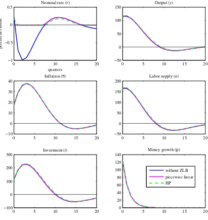
Figure 2 shows the impulse responses to the positive shock under the money growth
rule. Similar to the result obtained with the Taylor rule, the easing policy in the money
growth rule stimulates the economy and increase all of the variables indicated in Figure
2. The positive money growth shock lowers the nominal interest rate. This is called the
‘liquidity effect’, which is defined as the negative relationship between money growth and
the nominal interest rate. In the theoretical literature, the occurrence of the liquidity
effect depends negatively on the persistence of money growth rate (Christiano et al. 1997).
I set the money growth persistence, ρµ, at 0.5 to generate as strong a liquidity effect
as possible. The response of the nominal interest rate is very small relative to those
of the other macro variables. Both the dashed green line and the solid purple line
in Figure 1 indicate the impulse responses dealing with the non-negative constraint.
0 5 10 15 20 −1
−0.5 0 0.5
Nominal rate (r)
quarters
percent deviation
0 5 10 15 20
−50 0 50 100 150
Output (y)
0 5 10 15 20
−10 0 10 20 30 40
Inflation (π)
0 5 10 15 20
−50 0 50 100 150 200
Labor supply (n)
0 5 10 15 20
−100 0 100 200 300
Investment (i)
0 5 10 15 20
0 20 40 60 80 100 120 140
Money growth (µ)
[image:19.595.96.507.163.597.2]without ZLB piecewise linear HP
Table 2:
Variables Taylor rule
max(PW) max(HP) max(IRF)
yt 0.075585 0.081866 0.85686
it 0.12439 0.13501 0.579
nt 0.10742 0.11695 1.2241
πt 0.020795 0.021413 0.082309
max(PW): maximum responses with the ZLB by the piecewise linear solution; max(HP): maxi-mum responses with the ZLB by the HP algorithm; max(IRF): maximaxi-mum responses without the ZLB to monetary policy shocks for each variables.
Table 3:
Variables Money growth rule
max(PW) max(HP) max(IRF)
yt 115.3241 115.8718 117.2244 it 228.1931 233.1472 230.1629 nt 163.5437 164.3163 166.2422 πt 37.4943 36.7371 37.7284
max(PW): maximum responses with the ZLB by the piecewise linear solution; max(HP): maxi-mum responses with the ZLB by the HP algorithm; max(IRF): maximaxi-mum responses without the ZLB to monetary policy shocks for each variables.
7 quarters and reaches the lower bound again for 17 quarters. The nominal interest
rate could not ease significantly because of the ZLB. The result of this insignificant
easing in the nominal interest rate spills over and then lowers the response of the other
variables. However, the reductions in responses are extremely small. This is reflected by
the extreme closeness of the solid blue line, the solid purple line and the dashed green
line. Next I compare the effect of zero lower bound between the Taylor rule and the
money growth rule. First, I compare the maximum responses of four variables. Tables
2 and 3 indicate the maximum responses of yt, it, nt and πt to each monetary policy
shock. The columns labeled max(PW) and max(HP) indicate the maximum value of
responses to the monetary policy shock in the HP algorithm and the piecewise linear
solution. The colunmns of max(IRF) indicate the maximum value of responses to the
monetary policy shock without constraint. The result from max(PW) and max(HP) are
close to each other. In Table 2, the results from max(PW) and max(HP) are less than
Table 4: The Effects of ZLB indicate ∑
|IRF−ZIRF|/∑
|IRF|for each variables.
variables Taylor rule Money growth rule
Effects of ZLB PW HP PW HP
yt 80.4885% 78.2123% 1.6348% 4.2977%
it 74.3258% 71.8679% 1.0829% 4.5272%
nt 82.1438% 80.4424% 1.5695% 3.8598%
πt 70.6225% 69.5775% 1.0385% 3.1222%
close to max(IRF) in Table 3. Thus, the maximum responses to monetary policy shocks are more greatly affected by the non-negative constraint on the nominal interest rate
under the in Taylor rule than under the money growth rule.
Second, I compare the effect of the zero lower bound in impulse responses for 20
periods.
20
∑
t=0
|IRFt−PWt|/
20
∑
t=0
|IRFt| and
20
∑
t=0
|IRFt−HPt|/
20
∑
t=0 |IRFt|
Table 4 indicates that the effects of constraint are much larger under the Taylor rule
than the money growth rule. The responses with constraint were about 70%-80% of
the size of the responses without constraint under the Taylor rule. The responses with
constraint were about 1%-4% of the size of the responses without constraint under the
money growth rule.
3.3 Flexible wages
Next, I derive the impulse responses without the wage stickiness. Since there is no
stickiness in wage, the version of the Philips curve equation is substituted for the labor
supply equation from which the household’s first order conditions are derived. The
log-linearized version is
nt+σct=wt. (47)
Figure 3 indicates the impulse responses to the negative monetary policy shock under
the Taylor rule. Some standard responses without sticky wages become larger than the responses with sticky wages and others do not. The response of the nominal interest
rate with a flexible wages rate is smaller than that of the nominal interest rate with
0 5 10 15 20 −1
−0.5 0 0.5
Nominal rate (r)
quarters
percent deviation
0 5 10 15 20
−0.5 0 0.5 1
Output (y)
0 5 10 15 20
−0.2 0 0.2 0.4 0.6 0.8
Inflation (π)
0 5 10 15 20
−0.5 0 0.5 1 1.5
Labor supply (n)
0 5 10 15 20
−0.2 0 0.2 0.4 0.6
Investment (i)
0 5 10 15 20
−2.5 −2 −1.5 −1 −0.5 0
Policy shock (vr)
[image:22.595.95.510.159.597.2]without ZLB piecewise linear HP
Table 5:
variables Maximum responses Effects of ZLB
max(PW) max(HP) max(IRF) PW HP
yt 0.46998 0.5136 0.99972 42.2759% 38.4409%
it 0.3045 0.32513 0.43061 25.9485% 24.1256%
nt 0.67139 0.73371 1.4282 41.3739% 37.1486%
πt 0.45146 0.47694 0.62137 23.2359% 27.5527%
max(PW): maximum responses with the ZLB by the piecewise linear solution; max(HP): maxi-mum responses with the ZLB by the HP algorithm; max(IRF): maximaxi-mum responses without the ZLB to monetary policy shocks under flexible wages. The columns of Effects of ZLB indicate
∑
|IRF−ZIRF|/∑
|IRF|for each variable, where, the monetary policy rule is the Taylor type.
in some variables. The standard maximum response of inflation becomes much larger
than that with sticky wages. This feature is consistent with the study by Christiano et al. (2005) in that the nominal rigidities, especially the wage rigidity, contributes to the
initial dynamics of inflation.
The responses with the ZLB constraint become larger than those with sticky wage.
The intuitive reason for the reduction in the effects of the ZLB is that the inflation
dynamics becomes larger because of the absence of sticky wage. The inflation can abosorb
the effects of the constraint more than before since the dynamics of inflation become
larger. Table 5 provides the sticky wage versions of Tables 2, 3 and 4. First, the
maximum responses of variables with the constraint are more close to max(IRF) than
the case with sticky wages. Second, the effects of the constraint decrease in all variables.
Thus, the effects of monetary policy shock under the Taylor rule with frexible wages are larger than those with the sticky wages.
3.4 The persistency in policy shock under the Taylor rule
The persistency in policy shock under the Taylor rule, ρr, contributes to the dynamics
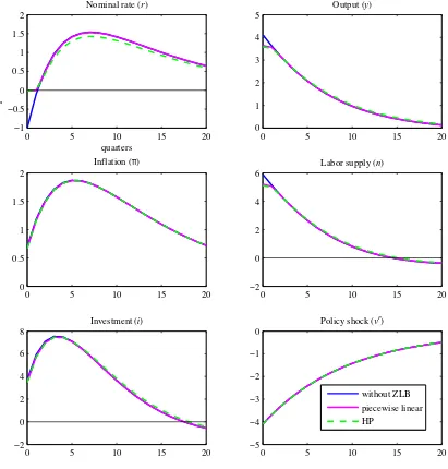
of the nominal interest rate. Figure 4 indicates the impulse responses when ρr is 0.9.
The impulse response of the nominal intrerest rate with the ZLB stays zero for initial periods, but it departs from zero earlier than the case without the ZLB. The responses
of other variables with the ZLB became close to those without the ZLB. An increase
in the persistence of policy shock lowers the negative response of the nominal interest
rate because high persistence of policy shock indicates that monetary easing continues
0 5 10 15 20 −1
−0.5 0 0.5 1 1.5 2
Nominal rate (r)
quarters
percent deviation
0 5 10 15 20
0 1 2 3 4 5
Output (y)
0 5 10 15 20
0 0.5 1 1.5 2
Inflation (π)
0 5 10 15 20
−2 0 2 4 6
Labor supply (n)
0 5 10 15 20
−2 0 2 4 6 8
Investment (i)
0 5 10 15 20
−5 −4 −3 −2 −1 0
Policy shock (vr)
[image:24.595.98.509.165.595.2]without ZLB piecewise linear HP
Figure 4: Impulse responses to monetary policy shocks under the Taylor rule when
ρr = .9. Solid blue line: the impulse response without the ZLB; Solid purple line: the
results indicate that an increase in the persistence of policy shock under the Taylor rule
dramatically mitigates the effects of ZLB through the reduction of the response of the
nominal interest rate.
4
Conclusion and Future Task
The main finding of this paper is that the influence of the ZLB on the effects of monetary
policy shock under the Taylor rule is larger than under the money growth rule in a typical
DSGE model. The reduction in the nominal interest rate is small compared to the money
growth shock. The ZLB constraint on the nominal interest rate has little effect on the
other variables because of the insignificant negative responses of the nominal interest
rate to money growth shocks. In other words, the ZLB does not affect the economy so
much because of the weak liquidity effect. However, this result is unrealistic because
there might be a strong liquidity effect in the actual economy. It is thus important to
use models that can generate a strong liquidity effect. This implication is related to the third analysis described herein, which assessed the effects of ZLB in high persistence of
shocks to Taylor rule. The ZLB might have a significant effect on the impact of monetary
policy shocks under the Taylor rule in models that generate strong liquidity effects even
though shock persistence is high.
Second, flexible wages reduce the effects of the ZLB and increase some variables’
responses. Wage stickiness affects the dynamics of inflation through the marginal costs
of the intermediate goods sector. A reduction in the stickiness of wages raises inflation
and then reduces the response of the nominal interest rate. A decrease in the response of
nominal rate of interest mitigates the amplification of the effects of anticipated bindings in
the HP algorithm, but this result does not necessally indicate that reduce wage stickiness is good method of decreasing the effects of the ZLB. This issue should be explored further
in the field of optimal monetary policy.
Third, the results obtained with the HP algorithm and those obtained with the
piecewise linear solution are close to each other in all analyses in this model.
Finally, these results are not necessarily consistent with the traditional IS-LM
liter-ature since monetary policy shocks affect the economy under some cases. This result
may indicate that the model cannot explain the real economy or that monetary policy
is effective even though the nominal interest rate cannot decrease further than zero. It
to search for a way to greatly reduce response of of the nominal interest rate to the
money growth shocks. The effects of monetary policy employing the Taylor rule might
become close to completely ineffective in such models. The liquidity effect might be more
important, because of the ZLB.
References
[1] Adam, K. and Billi, R. M. (2006) “Optimal Monetary Policy under Commitment
with a Zero Bound on Nominal Interest Rates,” Journal of Money, Credit and
Banking, Vol. 38, No. 7, pp. 1877-1905, October.
[2] Adam, K. and Billi, R. M. (2007) “Discretionary Monetary Policy and the Zero
Lower Bound on Nominal Interest Rates,”Journal of Monetary Economics, Vol. 54,
No. 3, pp. 728-752, April.
[3] Calvo, G A. (1983) “Staggered prices in a utility-maximizing framework,” Journal
of Monetary Economics, Vol. 12, No. 3, pp. 383-398, September.
[4] Christiano, L. J., Eichenbaum, M., and Rebelo, S. (2011) “When Is the Government
Spending Multiplier Large?” Journal of Political Economy, Vol. 119, No. 1, pp.
78-121.
[5] Christiano, L. J., Eichenbaum, M., and Evans, C. L. (1997) “Sticky price and limited
participation models of money: A comparison,” European Economic Review, Vol.
41, No. 6, pp. 1201-1249, June.
[6] Christiano, L. J., Eichenbaum, M., and Evans, C. L. (2005) “Nominal Rigidities and
the Dynamic Effects of a Shock to Monetary Policy,”Journal of Political Economy,
Vol. 113, No. 1, pp. 1-45, February.
[7] Eggertsson, G.B. and Woodford, M. (2003) “The Zero Bound on Interest Rates and
Optimal Monetary Policy,”Brookings Papers on Economic Activity, Vol. 34, No. 1,
pp. 139-235.
[8] Erceg, C. J., Henderson, D. W. and Levin, A. T. (2000) “Optimal Monetary Policy
with Staggered Wage and Price Contracts,” Journal of Monetary Economics, Vol.
46, No. 2, pp. 281-313, October.
[9] Fern´andez-Villaverde, J., Gordon, G., Guerr´on-Quintanan, P. A. and
Rubio-Ram´ırez, J. (2012) “Nonlinear Adventures at the Zero Lower Bound,” NBER Work-ing Papers 18058, National Bureau of Economic Research, Inc.
[10] Fujiwara, I., Sudo, N. and Teranishi, Y. (2010) “The Zero Lower Bound and
Mone-tary Policy in a Global Economy: A Simple Analytical Investigation,”International
[11] Guerrieri, L., and Iacoviello, M. (2013)“Occbin: A Toolkit to Solve Models with
Occasionally Binding Constraints Easily”, working paper, Federal Reserve Board
[12] Holden, T. and Paetz, M. (2012) “Efficient Simulation of DSGE Models with In-equality Constraints,” Quantitative Macroeconomics Working Papers 21207b, Ham-burg University, Department of Economics.
[13] Ida, D. (2013) “Optimal Monetary Policy Rules in a Two-Country Economy with a
Zero Bound on Nominal Interest Rates,”The North American Journal of Economics
and Finance, Vol. 24, No. C, pp. 223-242.
[14] Kato, R. and Nishiyama, S. (2005) “Optimal Monetary Policy When Interest Rates
Are Bounded at Zero,” Journal of Economic Dynamics and Control, Vol. 29, No.
1-2, pp. 97-133, January.
[15] Jung, T., Teranishi, Y. and Watanabe, T. (2005) “Optimal Monetary Policy at the
Zero-Interest-Rate Bound,”Journal of Money, Credit and Banking, Vol. 37, No. 5,
pp. 813-835, October.
[16] Nakajima, T. (2008) “Liquidity Trap and Optimal Monetary Policy in Open
Economies,” Journal of the Japanese and International Economies, Vol. 22, No.
1, pp. 1-33, March.
[17] Nakata, T. (2012) “Optimal Fiscal and Monetary Policy With Occasionally Binding Zero Bound Constraints,” manuscript, New York University.
[18] Nakov, A. (2008) “Optimal and Simple Monetary Policy Rules with Zero Floor on
the Nominal Interest Rate,” International Journal of Central Banking, Vol. 4, No.
2, pp. 73-127, June.
[19] Sims, C. A. (2002) “Solving Linear Rational Expectations Models,” Computational
Economics, Vol. 20, No. 1-2, pp. 1-20, October.
[20] Smets, F., and Wouters, R. (2003) “An Estimated Dynamic Stochastic General
Equilibrium Model of the Euro Area,”Journal of the European Economic
Associa-tion, Vol. 1, No. 5, pp. 1123-1175, 09.
[21] Taylor, J. B. (1993) “Discretion Versus Policy Rules in Practice,”