Loss Given Default Modelling: Comparative Analysis

Munich Personal RePEc Archive

Loss Given Default Modelling:

Comparative Analysis

Yashkir, Olga and Yashkir, Yuriy

Yashkir Consulting

27 March 2013

Online at

https://mpra.ub.uni-muenchen.de/46147/

Loss Given Default Modelling: Comparative Analysis

(pre-typeset version)

(Final version is published in "Journal of Risk Model Validation", v.7,No.1(2013))

Dr. Olga Yashkir

_{Dr. Yuri Yashkir}

Abstract

In this study we investigated several most popular Loss Given Default (LGD) models (LSM, Tobit, Three-Tiered Tobit, Beta Regression, Inated Beta Regression, Censored Gamma Regression) in order to compare their performance. We show that for a given input data set, the quality of the model calibration depends mainly on the proper choice (and availability) of explanatory variables (model factors), but not on the tting model. Model factors were chosen based on the amplitude of their correlation with historical LGDs of the calibration data set. Numerical values of non-quantitative parameters (industry, ranking, type of collateral) were introduced as their LGD average. We show that dierent debt instruments depend on dierent sets of model factors (from three factors for Revolving Credit or for Subordinated Bonds to eight factors for Senior Secured Bonds). Calibration of LGD models using distressed business cycle periods provide better t than data from total available time span. Calibration algorithms and details of their realization using the R statistical package are presented. We demonstrate how LGD models can be used for stress testing. The results of this study can be of use to risk managers concerned with the Basel accord compliance.

Contents

1 Introduction 2

2 Methodologies 3

3 Data, Explanatory Variables and Correlation Analysis 9

4 Comparative Model Analysis 12

5 Calibration Examples with the Best Fitting Results 18

6 Data Sensitivity and Stress Testing 23

7 Conclusions 26

8 References 27

1 Introduction

The goal of Loss Given Default (LGD) modelling is to produce simulated LGDs close to and as correlated with historical LGDs. Diculties with modelling depend directly on the specics of the data used and on the limitations of the models.

In recent years, the importance of modelling LGD has increased signicantly. The LGD model development, calibration, and implementation strategies have been analysed and summarized in several publications (Gupton, 2005), (Schuermann, 2004).

The predictive power of any LGD model depends, rst of all, on proper choice (and availability) of the model input parameters obtained from obligor's information. These (predictive) variables were analyzed and used for LGD model calibration in many publications. For example, the nine-factor model was analysed in (Gupton and Stein, 2002), the survey of LGD model factors is presented in (Friedman and Sandow, 2003). A case study of the modelling of bank loan LGDs where the primary factors (the period of loan origination, quality of the collateral, the loan size, and the length of the relationship with the obligor) were identied (Chalupka and Kopecsni, 2009). The link between default and recovery rates was investigated in (Altman et al., 2003), (Altman et al., 2004), (Altman, 2006a), (Altman, 2006b). The incorporation of the dependence between probabilities of default and recovery rates investigated by (Bade et al., 2011) demonstrated some improvement of the LGD model. A signicant impact of the uncertainty of model parameters on estimated LGDs was demonstrated in (Luo and Shevchenko, 2010). The inuence of the length of the LGD workout process on the level of estimated LGD can be signicant, as shown in (Gurtler and Hibbeln, 2011).

The portfolio credit risk model dependent on LGD was developed in (Hillebrand, 2006) and compared with several alternative LGD models. Calibration methods for LGD models applied to mortgage markets can be found in (van der Weija and den Hollandera, 2009). The results in (Bellotti and Crook, 2012) contain comparison of several models (Tobit, decision-tree model, beta transformation, fractional Logit, and the Least Square method). They demonstrated the importance of the inclusion of macroeconomic conditions (interest rates, unemployment levels, and earning index) for the LGD model stress testing. The paper (Yang and Tkachenko, 2012) proposes some empirical approaches for EAD/LGD modeling and provides technical insights into their implementation. Validation techniques and performance metrics for loss given default models were introduced by (Li et al., 2009).

An attempt to develop analytic formulas for downturn LGD estimation was done by (Barco, 2007). The downturn LGDs were considered as a 1/1000-year event with account of correlated PD and LGD. The paper by (Rosch and Scheule, 2007) developed a framework to stress sensitivities of risk drivers, and therefore a credit portfolio losses.

Given results of all the above research publications, the main question for a practitioner remains: what is the best model for LGD estimation? The goal of our research is to provide comparative tests of popular LGD estimation models, to analyze their performance, to calibrate the models on dierent data subsets, and, in addition, to provide recommendations on how test results can be used for the stress testing of LGDs.

We do not include data manipulation techniques. Based on some examples, we show how models can become sensitive to the choice of data.

2 Methodologies

The LGD models, analyzed and compared in this paper, are based on several dierent linear regression algorithms. A short description of the models is summarized in this section.

Censored Least Square Method

Given known historical LGD values _LGD⃗ ∗, coecients _x

k are derived using the Least Square

Method (LSM) by minimizing the following object function:

min

⃗x

∑

i

(yi(⃗x,r)−LGD∗i)

2

(1)

with

yi(⃗x,r) =x0+

n

∑

k=1

xk·rik (2)

where

rik is thekthpredictive parameter forith counterparty ,

xk is the coecient forkthpredictive parameter ,

x0 is a constant ("intercept").

The LGD for the debt facilityiis estimated as:

Censored Linear Regression (Tobit) Model

The Tobit LGD model is based on the latent "loss" parameter zi for each debt facility i

(see(McDonald and Mott, 1980)):

zi=yi+ϵ(σ) (4)

Here: ϵ(σ) is a normally distributed random driver with standard deviation σ, yi(⃗x,r) is the

linear combination of explanatory variablesrik as in (2).

The latent loss variablezi is a normally distributed random value with expected value ofyi and

standard deviation ofσ. Therefore, the probability of realization ofLGDi=scan be expressed

through the standard Gaussian functiong(·)as follows:

1

σ√2πexp

[ −1₂

(

s−yi

σ

)2] ≡ _σ1 ·g

(

s−yi

σ

)

(5)

Assuming that alls≤0 correspond toLGD= 0 and that alls≥1 correspond toLGD = 1we

can dene the probability functionPi(x)forLGDas follows:

Pi(x) =

    

P_i(0) ifx≤0

1

σ ·g

(x−y_i

σ

)

if0< x <1

P_i(1) ifx≥1

(6)

Where

P_i(0)= 1

σ·

∫ 0

−∞

g

(_z −yi

σ

)

dz=N(−yi

σ

)

(7)

P_i(1)= 1

σ·

∫ ∞

1

g

(

z−yi

σ

)

dz=N

(

−1−_σyi )

(8)

WhereN()is a standard normal cumulative distribution function.

The probability function(6)can be also presented in a more convenient form

Pi(z) =P

(0)

i ·δ(z) +P

(1)

i ·δ(z−1) +

1

σ·g

(

z−yi

σ

)

·(1−δ(z)−δ(z−1)) (9)

whereδ()is the standard delta-function.

Note that the probability(6)is also the function of model coecientsxk (k= 0 :n) and of the

LGD volatility σ which are the subjects of the model calibration. Expected LGD for ith _debt

facility is calculated asE[LGDi] =

∫1

0z·Pi(z)·dz. The result is

E[LGDi] =P

(1)

i + (1−P

(0)

i −P

(1)

i )·yi+σ

[

g(yi σ

) −g

(

−1−_σyi )]

. (10)

The cumulative LGD probability can be calculated using (6) asQ(LGDi) =

∫LGDi

0 Pi(z) dz :

Qi(LGD) =

      

P_i(0) ifLGD= 0

N(LGD−y_i

σ

)

if0< LGD <1

1 ifLGD= 1

Theηth_{percentile of the modelled LGDs (LGD}(η)

i ) is the solution of the equationQi(LGD) =η.

LGD(_iη)=

    

0 ifη < P_i(0)

yi+σ·N−1(η) ifPi(0)< η <1−P

(1)

i

1 ifη >1−P_i(1)

(12)

The calibration of the Tobit model consists in nding model coecients xk (k = 0 : n ) and

LGD volatility σ by best t of the model (with predictive parameters rik) to historical data

LGDi (k = 1 : n, i = 1 : J). If we consider the input data sample as a set of independent

"measurements" then the best model t is obtained by maximizing the total probability of getting this input data set:

ˆ

P(⃗x, σ) =

J

∏

i=1

Pi(LGDi) (13)

which is equivalent to minimization of the following objective function

Φ(⃗x, σ) =−

J

∑

i=1

logPi(LGDi) (14)

For numerical optimization we employ the BroydenFletcherGoldfarbShanno (BFGS) method (for solving non-linear optimization problems without constraints).

The linear dependence of the function (2) on explanatory variablesrkj may not be sucient to

describe the cause-eect link ofLGDj torkj. It is possible to increase exibility of the model

by including a quadratic term, such that

yi(⃗x,r) =x0+

n

∑

k=1

(

x2k−1·r_ik+x2_k·r

2

ik

)

(15)

Note that number of model coecients for the nonlinear Tobit model is2n+ 1.

Censored Linear Regression Three-Tiered Tobit Model

Since processes causing LGD to be zeroes or ones may have a dierent nature compared to processes where 0 < LGD < 1, we introduce in this section a three-tiered model. The LGD

estimator is introduced in this case in the following linear form:

yi(0)(⃗x,r) = n

∑

k=1

xk·rik+xn+2 (16)

y(_ic)(⃗x,r) =

n

∑

k=1

xk+n+2·rik+x2n+4 (17)

y_i(1)(⃗x,r) =

n

∑

k=1

where components of the model coecient vector⃗xhave the following meaning: ⃗x=                                 

x1...n coecients for theLGD= 0model

xn+1 σ0 for theLGD= 0model

xn+2 intercept for theLGD= 0model

x(n+3)...(2n+2) coecients for modeling0< LGD <1

x2n+3 σfor the0< LGD <1 model

x2n+4 intercept for the0< LGD <1model

x(2n+5)...(3n+4) coecients for theLGD= 1model

x3n+5 σ1 for theLGD= 1model

x3n+6 intercept for theLGD= 1model

(19)

This LGD model is based on the following probability function for anith_facility:

Pi(z) =

        

p(0)_i ifz= 0

κ σg

(

z−_y(c)

i

σ

)

if0< z <1

p(1)_i ifz= 1

(20) where               

p(0)_i =N

( −y (0) i σ0 )

p(1)_i =κ·N

( −1−y

(1) i

σ1

)

κ =N

(

y(0)_j σ0

) [

N

( −1−y

(1) i σ1 ) +N (

1−_y(c)

i σ ) −N ( −y

(c) i

σ

)]−1

(21)

Hereκis a normalization factor.

The model coecients ⃗x can be found as a result of the maximization of the following

log-likelihood function:

H(⃗x) =∑

i

logPi(LGDi) (22)

Using calibrated model coecients one can estimate expected LGDs:

LGDi=p(1)i +y

(c)

i κ

[

N

(

1−y(_ic) σ

) −N

( −y

(c)

i σ )] +σκ [ N (

y(_ic) σ

) −N

(

1−y_i(c) σ

)] (23)

Inated Beta Regression Model

The Inated Beta Regression LGD model (Pereira and Cribari-Neto, 2010) is based on the following probability function for anith_facility:

Pi(z) =

     Pi

0 ifz= 0

(1−Pi

0−P1i)·f(z;µj, ϕi) if0< z <1

Pi

1 ifz= 1

(24)

where

f(z;µj, ϕi) = Γ(ϕ

i₎

Γ(µi_ϕi_)Γ((1−µi_)ϕi₎z µi_ϕi₋₁

(1−z)(1−µi)ϕi−1

with0< µi_{<1 andϕ}i_>0(µi _{being the mean value).}

GivenPi

0,P1i,µi, andϕi, one can calculate (using (24)) probabilitiesPi(LGDi)of gettingLGDi

values. In order to establish a connection between explanatory variablesri

k of debt facilities and

expected facility LGDs, the following four linear predictors are introduced:

log P

i

0

1−Pi

0

=a0+

n

∑

k=1

x0krki (26)

log P

i

1

1−Pi

1

=a1+

n

∑

k=1

x1krki (27)

log µ

j

1−µj =aµ+ n

∑

k=1

xµ_krj_k (28)

log ϕ

i

1−ϕi =aϕ+ n

∑

k=1

xϕ_krik (29)

Here vectors ⃗x(0,1,µ,ϕ) _{and a}

(0,1,µ,ϕ) are model coecients and intercepts, respectively. The

model calibration consists of nding coecients and intercepts by maximizing the following log-likelihood (objective) function:

H =∑

i

log(Pi(LGDi)) (30)

Using calibrated model one can estimate expected LGD for anith_{debt facility:}

E[LGD]i=

∫ 1

0

zPi(z)dz=P1i+

1−Pi

0−P1i

(1 + exp(−(aµ+∑nk=1x

µ k·rki)))

(31)

The log-likelihood function (30) can be split as follows:

H =H01+Hβ (32)

whereH01(⃗x(0), ⃗x(1))andHβ(⃗x(µ), ⃗x(ϕ))can be optimized independently:

H01=

LGDi=0

∑

i

log(P0(⃗x(0))) +

LGDj=1

∑

i

log(P1(⃗x(1)))

+

0<LGDi<1

∑

i

log(1−P0(⃗x(0))−P1(⃗x(1)))

(33)

Hβ=

0<LGDi<1

∑

i

logf(LGDi;⃗x(µ), ⃗x(ϕ)) (34)

Beta Linear Regression Model

If0 < LGD < 1 thenP0 =P1 = 0, reducing the problem to a general Beta Regression Model

(34)1_{. This model (34) can be also used if all LGDs are scaled asLGD}∗

=LGD·(β−α) +α

, calibration performed using LGD∗ , and values of

LGD∗

est (estimated on the basis of this

calibration) are scaled back as LGDest = (LGD∗est−α)/(β−α). The Beta Regression Model

was tested using the BetaReg library function of the R statistical package.

Censored Gamma Linear Regression Model

The Censored Gamma LGD model (Sigrist and Stahel, 2010) is based on the following probability function for anith_facility:

Pj(z;ξ, α, θi) =

    

Ψ(ξ, α, θi) ifz= 0

γ(z+ξ, α, θi) if0< z <1

1−Ψ(1 +ξ, α, θi) ifz= 1

(35)

where _{

γ(u;α, θi) = _θiΓ(1α)uα

−1

e−u

θi (gamma distribution)

Ψ(u;α, θi) =

∫u

0 γ(x;α, θi)dx (cumulative gamma distribution)

(36)

withu >0,α >0, andθi>0.

Givenξ,α, andθi, using (35), one can calculate probabilitiesPi(LGDi)of gettingLGDivalues.

In order to establish a connection between explanatory variablesri

kof debt facilities and expected

facility LGDs, the following linear predictors are introduced:

    

logα=α∗

logξ=ξ∗

logθi=x0+∑n_k=1xkrki

(37)

Here xk are model coecients (including the intercept x0). The model calibration involves

nding coecients and parametersα∗

,ξ∗

by maximizing the following log-likelihood (objective) function:

H(ξ∗

, α∗

, ⃗x) =∑

i

logPi(LGDi;ξ, α, θi) (38)

Using the calibrated model one can estimate expected LGD for anith_{debt facility:}

E[LGD]i₌∫

1

0

zPj(z;ξ, α, θi)dz (39)

=α·θi(Ψ(1 +ξ,1 +α, θi)−Ψ(ξ,1 +α, θi))

+ (1 +ξ) (1−Ψ(1 +ξ, α, θi))−ξ(1−Ψ(ξ, α, θj))

The Censored Gamma Regression model was tested using the R-coded function developed by Yashkir Consulting.

3 Data, Explanatory Variables and Correlation Analysis

Data used for LGD model calibration

The data set All Data represents all available data in an internal or an external database used for the LGD model development and calibration. In our analysis, All Data is the S&P LossStats data (2011 update, 4275 cases) of defaulted facilities. Only results of analysis based on this data are presented in this paper.

The Peaks Data is the LGD data related to the time periods of the business cycle when the number of defaults and losses is signicantly higher than the average default and losses values. We chose years1990−1991as the Peak 1, years2001−2002as the Peak 2, and years2008−2009

as Peak 3. All three peaks have distinctly high levels of defaults and losses (shown in Fig.1, based on the recent report from S&P (Standard&Poor's, 2012)). During peaks of the cycle, global market and credit conditions are dierent from the quiet periods of the cycle, therefore, the most important predictive factors are correlated at a higher level with the historical LGD data collected for these time periods.

Figure 1: Total Debt Outstanding and Total Number of Defaults

Bankruptcy and Peaks Data represents the bankruptcy data from the peak periods.

Explanatory Variables/Factors

The explanatory variables were chosen based on how they are correlated with the LGDs based on the collected historical data. The proper choice of data and instrument types are very important for good performance of the models, therefore, the model calibration was tested for several groups based on instrument types.

The following main ve factors (explanatory variables) were used: Ranking (denes rank in the capital structure, the more senior the instrument, the higher the recovery rate), Debt Cushion (amount/percentage of debt below a defaulted instrument), Principal Above (amount of debt above a defaulted instrument), Eective Interest rate (prepetition rate at the time the last coupon was paid), and Spread.

We introduce also three additional factors (dependence on industry, on the type of collateral, and on the facility ranking): Industry mean LGD, Collateral mean LGD, Ranking mean LGD.

The choice of additional factors makes the model dependent on industry, collateral type, and ranking, for which no numerical predictive parameters are available. These additional factors were calculated as the mean of all LGD values for a given industry, for a given collateral type, and for a given ranking. For example, Industry Mean LGD is the mean value of all LGDs for the cases related to a specied industry. This value is added as an additional factor to all cases belonging to the specied industry. The same was done for Collateral Mean LGD and Ranking Mean LGD. The Collateral Mean LGD depends on a type of the collateral and it denes the mean of all cases for this type of collateral.

Correlation Analysis

Table 1: Correlation between factors and LGD (All Data, for dierent instruments)

Ranking Debt Principal Eective Spread Industry Cushion Above Interest Rate meanLGD Senior Unsecured Bonds -0.056 -0.071 -0.023 0.243 0.267 0.399 Revolving Credit 0.061 -0.299 0.027 -0.016 0.035 0.193 Term Loan 0.180 -0.347 0.191 0.016 0.059 0.208 Sr. Subordinated Bonds -0.043 -0.143 0.087 -0.024 0.038 0.269 Subordinated Bonds -0.004 0.023 0.019 -0.133 -0.144 0.205 Senior Secured Bonds 0.146 -0.403 0.202 0.146 0.173 0.281 Jr. Subordinated Bonds 0.268 0.043 -0.273 0.215 -0.007 0.516 Other 0.713 -0.652 0.589 0.280 0.545 0.260

All Instruments 0.348 -0.442 0.367 0.227 0.359 0.272

Collateral Ranking Original Principal Acclaimed Total mean LGD mean LGD Amount Default Amount Amount Debt Senior Unsecured Bonds 0.000 -0.078 0.132 0.001 0.147 -0.102 Revolving Credit 0.188 0.060 0.096 0.092 n/a 0.076 Term Loan 0.187 0.176 0.032 -0.009 n/a -0.065 Sr. Subordinated Bonds 0.106 -0.019 0.001 0.054 0.062 -0.053 Subordinated Bonds -0.010 0.008 0.118 -0.022 0.048 0.091 Senior Secured Bonds 0.209 0.158 0.027 0.017 0.066 -0.133 Jr. Subordinated Bonds 0.000 0.173 0.337 -0.058 0.135 0.224 Other 0.761 0.617 0.755 0.604 n/a 0.840

All Instruments 0.507 0.458 0.364 0.065 0.020 0.132

If all instrument types are considered together, the correlation between Instrument type mean LGDs with all LGDs is equal to 0.5103.

Table 2: Peak Data (years1990−1991; 2001−2002; 2008−2009), correlation between factors

and LGD

Ranking Debt Principal Eective Spread Industry Cushion Above Int.Rate meanLGD Senior Unsecured Bonds -0.076 -0.006 -0.016 0.301 0.315 0.484 Revolving Credit -0.032 -0.345 0.105 -0.153 0.071 0.262 Term Loan 0.050 -0.278 -0.044 -0.065 0.118 0.326 Sr. Subordinated Bonds 0.092 -0.221 -0.034 -0.164 -0.022 0.141 Subordinated Bonds 0.040 -0.038 0.127 -0.119 -0.135 0.162 Senior Secured Bonds 0.328 -0.463 -0.011 0.211 0.211 0.255 Jr. Subordinated Bonds 0.235 -0.088 0.286 -0.194 -0.225 0.310 Other 0.664 -0.699 0.596 0.815 0.919 0.676

All Instruments 0.292 -0.421 0.321 0.228 0.386 0.322

Collateral Ranking Original Principal Df. Acclaimed Total mean LGD mean LGD Amount Amount Amount Debt Senior Unsecured Bonds 0.000 -0.096 0.083 0.062 0.166 -0.058 Revolving Credit 0.181 -0.035 0.234 0.214 n/a 0.148 Term Loan 0.187 0.035 0.062 0.031 n/a -0.052 Sr. Subordinated Bonds 0.035 0.108 0.062 0.004 0.047 -0.034 Subordinated Bonds 0.091 0.025 -0.051 0.023 0.065 0.140 Senior Secured Bonds 0.312 0.323 0.133 0.100 0.193 -0.197 Jr.Subordinated Bonds 0.000 0.105 -0.070 -0.043 0.179 0.142 Other 0.935 0.638 0.472 0.568 n/a 0.586

In the case of Peak Data, if all instrument types are considered together, the correlation be-tween Instrument type mean LGDs with all LGDs is equal to 0.470. The comparison of the correlation level when using All Data and when using Peak Data, demonstrates the following:

1) Correlations of historical LGDs with Industry Mean LGD (mean of historical LGDs for a specied industry) are high for all instruments (from 14% to 68%),

2) Changes in correlation level are clearly seen when comparing All Data correlation results and Peak Data correlation results. The absolute values of correlation are higher for the Peak Data results. For example, Revolving Credit correlation with Debt Cushion is equal to -0.299 when using All Data, and it is equal to -0.345 when using Peak Data,

3) The signicance of Spread, Eective Interest rate and Total Debt factors increases during cycle peaks (as expected) due to the inuence of macroeconomic conditions increasing in cycle peaks.

The correlation level analysis demonstrates that sets of signicant factors (explanatory variables) are dierent for dierent instruments (Table 3). In this table, the most signicant explanatory variables are marked for each instrument. They were chosen based on the criteria that absolute values of correlations exceed 10%.

Table 3: Marked cells: absolute values of correlations(factor,LGD) exceed 10%

Ranking Debt Principal Eective Spread Industry Collateral Ranking Cushion Above Int. Rate mean LGD mean LGD mean LGD Revolving Credit

Term Loan Sr.Unsec. Bonds Sr.Sec. Bonds Sr.Sub. Bonds Sub. Bonds Jr.Sub. Bonds

The Spread Data was not always available, therefore, we did not include Spread into the calibra-tion of models. Based on the similarity of the factor sets, there are three groups of instruments that should be calibrated together:

Group A: Term Loan and Revolving Credit, Group B: Senior Unsecured,

Group C: Senior Secured Bonds, Senior Subordinated Bonds, Subordinated Bonds, and Junior Subordinated Bonds.

Note, that for testing purposes, we considered Senior Secured Bonds separately, but the obtained results did not show visible improvement in calibration criteria.

4 Comparative Model Analysis

Criteria for the Methodology Analysis

The Goodness-of-Fit and the model LGD Correlation were chosen as the criteria for the method-ology performance analysis. As a measure of Goodness-of-Fit (G) we use the following parameter

(often called "the coecient of determination")

G= 1− M SE

whereM SEis the mean square error (model versus historical LGD), andvarLGDis the variance

of the input data. The interpretation of the Goodness-of-Fit parameter Gis as follows. For a

"naïve" model, where predicted values of the model LGD are equal to the mean historical LGD, we would haveM SE=varLGDandG= 0(the model "t" is not better than "naïve" model).

On the other hand, if a model provides prediction such thatM SE≪varLGD (ideal case) then G∼1(a very good t). UsingM SE as a criterion of the t quality might be misleading. In the

following sections we will use the Gparameter as a criterion for comparison of dierent models

(values ofM SE and/or values of mean absolute error (M AE) are presented for convenience).

The model LGD Correlation (ρ), dened as the correlation between historical and simulated

LGDs, is also used for model comparison.

Calibration Details

This section describes the procedures, the R-functions used, and specic calibration approaches. Codes for Tobit, Inated Beta, and Gamma Reg models were developed by Yashkir Consulting using the statistical R package. Additional applications were developed in Python.

Least Square method: The library function in R provides solving of the problem (1)

Q=lsfit(r, ⃗L, ...) (41)

where r is the matrix of explanatory variables for a given set of defaulted cases, and L⃗ is the

vector of observed LGDs. From the output object (list)Qwe nd the following: the coecient

vector⃗x =Q1 (including intercept x0), the array of residuals⃗δ =Q2, and the modelled LGD

Li−δi for theithcase.

Object function minimization: The library function in R provides solving of the problem (14) (Tobit model):

Q=optim(⃗z,Φ(⃗z), ...) (42)

From the output object (list) we nd the coecient vector⃗z= (⃗x, σ) =Q1 .

Maximization of the log-likelihood function: The library function in R provides solving of the problem (22) (Three-Tiered Tobit model):

Q=optim(⃗x,−H(⃗x), ...) (43)

From the output object (list) we nd the coecient vector⃗x=Q1 .

Maximization of the log-likelihood function for Beta Regression: The library function in R provides solving of the problem (34):

Q=betareg(F ORM U LA, link= ”logit”, data=DAT A) (44)

where F ORM U LA is the following string: ”LGD ∼ N1+N2+...” and DAT A is the table

containing input data in the following format:

Table 4: Input data

N₁ N₂ ... LGD V11 V12 ... LGD1∗

V21 V22 ... LGD2∗

where N_i (predictive variable names) and LGDare column headers; Vji and LGDj∗ are

corre-sponding numerical values for every jth_transaction 2_{. From the output object (list) Qwe nd}

the following: the coecient vector⃗x=Q1 (including interceptx0), and the array of residuals

⃗δ=Q2.

The modelled LGD for ith _{case is LGD}mod

i =

LGD∗

i−δ_i−α

β−α . In general, an LGD of any j

th

transaction is estimated as

LGDj =

1

1 +e−_yj (45)

with the predictor

yj =x0+

∑

k

xk·rjk (46)

Term Loan and Revolving Credit (Group A)

Results of the methods performance are presented below for the Instrument Group A (Term Loan and Revolving Credit)3_.

Table 5: Instrument Group A (Factors: Debt Cushion , Industry mean LGD, Collateral mean LGD)

Data All Data Peak Data Bankruptcy Bankruptcy Model data peaks data

Tobit

G= 0.1538 0.2242 0.1768 0.2167

M AE= 0.1977 0.2246 0.2123 0.2282

ρ= 0.3932 0.4745 0.4215 0.4666 Least Square

G= 0.1658 0.2341 0.1893 0.2280

M AE= 0.2021 0.2262 0.2157 0.2294

ρ= 0.4072 0.4838 0.4349 0.4772 Inated Beta

G= 0.1568 0.2254 0.1817 0.2157

M AE= 0.2036 0.2325 0.2201 0.2352

ρ= 0.3955 0.4798 0.4274 0.4691

BetaReg

G= 0.1615 0.2311 0.1857 0.2251

M AE= 0.2085 0.2305 0.2214 0.2337

ρ= 0.4062 0.4836 0.4340 0.4771 GammaReg

G= 0.1537 0.2239 0.1767 0.2164

M AE= 0.1976 0.2245 0.2122 0.2281

ρ= 0.3932 0.4743 0.4215 0.4664

The best t for these instruments was obtained using LSM and BetaReg. Two important obser-vations can be made for the case of Term Loans and Revolving Credits:

1) The best t for all sets of data was achieved by using Least Square Method (LSM),

2_{Values LGD}∗

j are scaled values of real LGDs as follows: LGD

∗

j = LGDj∗(β−α) +α to ensure that 0< α≤LGD∗

j ≤β <1.

3_{Revolving line of credit is an agreement by a bank to lend a specic amount to a borrower, and to allow}

2) The best t was achieved on Peak Data using LSM and Beta Reg (Goodness-of-Fit is ap-proximately 0.23 and Correlation is apap-proximately 0.47).

In peak conditions of the cycle, the predictive power of the chosen facility parameters increases, which results in higher values of Goodness-of-Fit and Correlations for Peak Data. This out-come of comparative tests for dierent calibration models clearly indicates that success of LGD modelling depends mainly on availability (and proper choice) of explanatory variables and on data quality, but not on tting techniques.

Senior Unsecured (Group B)

Senior Unsecured transactions (Instrument Group B) do not have any collateral. According to the correlation matrices (Table 1 and Table 2), main parameters that are highly correlated with the historical LGDs are Industry Mean LGD and the Eective Interest Rate4_{. Therefore, in case}

of Senior Unsecured the main factor dening the LGD level at default is the industry cluster to which the facility belongs.

4_{Eective Interest Rate, as by the S&P denition is the prepetition rate at the time the last coupon was}

Table 6: Instrument Group B (Factors: Industry mean LGD, Eective Interest Rate (EIR))

Data All Data Peak Data Bankruptcy Bankruptcy

Model Data Peaks Data

Tobit Industry.meanLGD

G= 0.1460 0.2220 0.2146 0.2692

ρ= 0.3894 0.4783 0.4710 0.5297

Industry.meanLGD and EIR

G= 0.1691 0.2479 0.2423 0.3021

ρ= 0.4180 0.5048 0.4994 0.5601 Least Square

Industry.meanLGD

G= 0.1595 0.2350 0.2295 0.2856

ρ= 0.3985 0.4836 0.4782 0.5332 Industry.meanLGD and EIR

G= 0.1825 0.2627 0.2562 0.3208

ρ= 0.4264 0.5115 0.5054 0.5653

Inated Beta Industry.meanLGD

G= 0.1562 0.2199 0.2206 0.2658

ρ= 0.4000 0.4871 0.4816 0.5379 Industry.meanLGD and EIR

G= 0.1775 0.2463 0.2471 0.2963

ρ= 0.4279 0.5161 0.5086 0.5681 BetaReg

Industry.meanLGD

G= 0.1574 0.2335 0.2275 0.2843

ρ= 0.3972 0.4831 0.4774 0.5334

Industry.meanLGD and EIR

G= 0.1808 0.2614 0.2548 0.3193

ρ= 0.4255 0.5112 0.5052 0.5653 GammaReg

Industry.meanLGD

G= 0.1457 0.2216 0.2142 0.2686

ρ= 0.3893 0.4783 0.4709 0.5296 Industry.meanLGD and EIR

G= 0.1688 0.2474 0.2418 0.3013

ρ= 0.4179 0.5047 0.4994 0.5600

The Senior Unsecured case is suciently dicult to model due to the fact that the strongest dependency is only on Industry Mean LGDs. Two important observations can be made for the case of Senior Unsecured:

1) The best t for all sets of data is done again using Least Square Method (LSM),

2) The best t was achieved on Bankruptcy Peak Data using LSM and Beta Reg (Goodness-of-Fit is approximately 0.32 and Correlation is approximately is 0.57).

con-ditions of the cycle, the industry becomes even more important. It should be noted that for this group of instruments, calibrated on Bankruptcy Peak Data, the Tobit and GammaReg models also provide suciently good t (Goodness-of-Fit is approximately 0.30, and Correlation is approximately 0.56). For contracts with xed interest rates (if default data contains this rate) the Eective Interest Rate can also be used for calibration.

Senior Secured, Senior Subordinated, Subordinated, and Junior Subordinated bonds (Group C)

For the Instrument Group C (Senior Secured, Senior Subordinated, Subordinated, and Junior Subordinated bonds), according to the correlation matrices (Table 1 and Table 2), the main parameters that are highly correlated with the historical LGDs are: Debt Cushion, Principal Above, Eective Interest Rate, Industry Mean LGD, Collateral Mean LGD, Ranking Mean LGD.

Table 7: Instrument Group C (Factors: Debt Cushion, Principal Above, Eective Interest Rate, Industry Mean LGD, Collateral Mean LGD, Ranking Mean LGD)

Data All Data Peak Data Bankruptcy Bankruptcy

Model Data Peaks Data

Tobit

G= 0.2420 0.2086 0.3818 0.3361

ρ= 0.4998 0.4633 0.6235 0.5858

Least Square

G= 0.2520 0.2161 0.3904 0.3429

ρ= 0.5017 0.4633 0.6245 0.5843 Inated Beta

G= 0.2406 0.2012 0.3660 0.3192

ρ= 0.4995 0.4623 0.6223 0.5872 BetaReg

G= 0.2500 0.2123 0.3877 0.3358

ρ= 0.5013 0.4605 0.6235 0.5794 GammaReg

G= 0.1998 0.2141 0.2955 0.2772

ρ= 0.4551 0.4714 0.5515 0.5383

The Instrument Group C model strongly depends on Debt Cushion, Principal Above, Industry mean LGD, Collateral mean LGD, Ranking mean LGD. The Eective Interest Rate also can be used if available. Two important observations can be made for this case:

1) The best t for all sets of data is done again using Least Square Method (LSM),

2) The best t was achieved on Bankruptcy Data using LSM and Beta Reg (Goodness-of-Fit is approximately 0.39, and Correlation is approximately 0.63).

5 Calibration Examples with the Best Fitting Results

The results presented in this section are the best t as described above. The marker (***) in Tables 8, 9, 10, indicates the most important factors. Results show that chosen factors for all three groups were properly chosen and are the important factors for the simulation.

Term Loans plus Revolving Credit (Group A)

The best t was obtained with Peak Data using LSM and Beta Reg. It should be noted (in addition to the criteria used) that the mean of the historical LGDs (equal to 0.247) and the mean of the simulated LGDs (equal to 0.250 for LSM, and equal to 0.258 for BetaReg) are very close. This is a supporting factor for the models' results.

Table 8: Results for the best t for cases of Term Loans and Revolving Credit

Term Loans and Revolving Credits

BetaReg, Peaks Data Least Square, Peaks Data Parameter Coecients Pr(>|z|) Parameter Coecients (Intercept) -1.40 < 2e-16 *** (Intercept) -0.19 Debt Cushion -0.70 4.22e-16 *** Debt Cushion -0.35 Industry meanLGD 2.57 < 2e-16 *** Industry meanLGD 1.25 Collateral meanLGD 0.78 7.21e-04*** Collateral meanLGD 0.39

G= 0.2311 0.2341

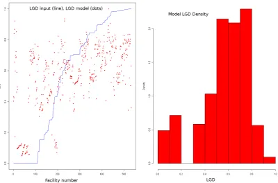
Figure 2: Modelling results for calibration on the Term Loans plus Revolving Credit data (G= 0.2341, M AE= 0.2262)

Figure 3: Model LGD versus historical LGDs (All Data, LSM,G= 0.1658,ρ= 0.4072)

around the diagonal line.

The histogram of the simulated LGDs is presented on Figure 2, right. The simulated LGD values are concentrated around the mean LGD value.

Senior Unsecured (Group B)

The best t was obtained for Bankruptcy Peak Data using LSM and Beta Reg. In addition to the tting quality criteria used, it is worth mentioning that the mean of the historical LGDs (equal to 0.5617) and the mean of the simulated LGDs (equal to 0.5616 for LSM, and is equal to 0.5583 for BetaReg) are very close. This is a supporting factor for the models' results.

Table 9: Results for the best t for Senior Unsecured cases

Senior Unsecured, Bankruptcy Peak Data

BetaReg Least Square

Parameter Coecients Pr(>|z|) Parameter Coecients (Intercept) -1.38 < 2e-16 *** Intercept -0.21 Eective.Interest.Rate 5.85 1.67e-07 *** Eective.Interest.Rate 2.94 Industry.meanLGD 2.34 < 2e-16 *** Industry.meanLGD 1.22

G= 0.3193 0.3208

M AE= 0.2564 0.2507

Figure 4: Fitting results for Senior Unsecured data set (G= 0.3208,M AE = 0.2507)

The historical LGDs and the model simulated LGDs (model LSM) are presented in Figure 4, left. Simulated LGD histogram is presented in Figure 4, right. There is concentration of the simulated values around the mean value as expected. Simulated LGDs (dots) reect the general trend of historical LGDs (solid line).

Senior Secured, Senior Subordinated, Subordinated, and Junior Subordinated Bonds (Group C)

Table 10: Results for the best t for the Instrument Group C

Bankruptcy Data

BetaReg Least Square

Parameter Coecients Pr(>|z|) Parameter Coecients (Intercept) -0.98 < 2e-16 *** Intercept 0.06 Principal Above 0.23 0.00129 ** Principal Above 0.16 Debt Cushion -0.72 8.0e-14 *** Debt Cushion -0.36 Eective Interest Rate -0.51 0.43069 Eective Interest Rate -0.24 Industry mean LGD 1.55 3.9e-16 *** Industry mean LGD 0.76 Collateral mean LGD 1.47 < 2e-16 *** Collateral mean LGD 0.81 Ranking.meanLGD -0.19

G= 0.3877 0.3904

M AE= 0.2381 0.2335

All chosen factors, except EIR, are shown as important.

Figure 5: Fitting results for the Instrument Group C (G= 0.3904,M AE= 0.2335)

The historical LGDs (solid line) and the model simulated LGDs (dots, LSM model) are presented in Figure 5, left. The histogram of simulated LGDs is shown in Figure 5, right. The results show good agreement between the simulated and the historical LGDs. The "cloud" of simulated values follows the historical LGDs.

Summary of Calibration Examples on All Data set

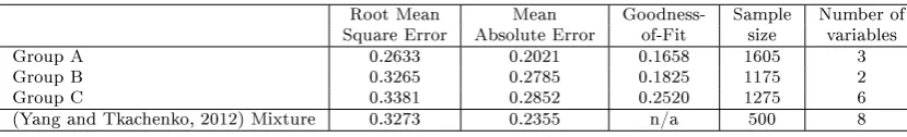
Table 11: Summary of Calibration Examples on the All Data set

Root Mean Mean Goodness- Sample Number of Square Error Absolute Error of-Fit size variables

Group A 0.2633 0.2021 0.1658 1605 3

Group B 0.3265 0.2785 0.1825 1175 2

Group C 0.3381 0.2852 0.2520 1275 6

(Yang and Tkachenko, 2012) Mixture 0.3273 0.2355 n/a 500 8

In the last row of Table 11, the results of the LGD "Mixture" model test by Yang and Tkachenko (Yang and Tkachenko, 2012) are presented for comparison. In their tests, the authors explored several models (Logit raw, HL logit, Logit, Least-squares logit, Naive Bayes, Mixture, and Neural Network) and found that the "Mixture" model has the lowest tting error. The results of our tests provide a similar or better level of tting errors.

Finally, as an example, we compare calibration results for groups A and C with a "naïve" model where the "model" LGDs are dened as historical average LGD.

Table 12: Comparison of the linear regression model results with "naïve" model

Mean Absolute Error G

Group A

Linear Regression 0.2021 0.1658 "Naïve" model 0.2365 0.0006 Group C

Linear Regression 0.2852 0.2520 "Naïve" model 0.3549 0.0008

Results presented in Table 12 demonstrate clearly advantages of using the Goodness-of-Fit pa-rameterGas a criterion for model comparison. For example, in case of the group A the MAE

changes from 23.65% to 20.21% only, but the Goodness-of Fit changes dramatically from 0.06% to 16.58%.

6 Data Sensitivity and Stress Testing

Data Sensitivity Test

Figure 6: Results for Senior Unsecured with adjusted data, Bankruptcy Peak initial data (G= 0.2963, M AE= 0.1796)

Stress Testing for LGDs

The approach of the LGD stress testing comes naturally from the results of our analysis of models and data. The stress test procedure is as follows:

1) Derive model coecients for peaks periods using the Peaks Data and/or data for each peak separately. These coecients emphasize the peak of crisis period in the the business cycle conditions.

2) Run simulations of All Data LGDs using these peak related coecients.

Figure 7: Stresstesting of LGDs: All Data calibration (solid line), Bankruptcy Data calibra-tion (dots)

Figure 8: Stresstesting of LGDs. The All Data calibration (solid line), Bankruptcy Data calibration (solid thin line), Bankruptcy Peaks Data calibration (open dots).

Our approach for the estimation of downturn LGDs does not require any additional model assumptions such as analytic approach by (Barco, 2007) or the parameter sensitivity approach by (Rosch and Scheule, 2007). The approach naturally follows the chosen model calibration procedure and the data choice.The downturn LGDs are estimated based on the chosen data subset consistent with the downturn conditions in the business cycle. If a nancial institution does not have enough data for Peaks Data set, then the external data for peaks periods can be used (following specic Basel II regulations). The external data that contains all available cases provide the data for the peak/stress LGD calibration.

7 Conclusions

Several most popular LGD models (LSM, Tobit, Three-Tiered Tobit, Beta Regression, Inated Beta Regression, Censored Gamma Regression) were tested on real data in order to compare their performance. Model factors were chosen based on the amplitude of their correlation with historical LGDs of the calibration data set. Numerical values of non-quantitative parameters (industry, ranking, type of collateral) were introduced as their LGD averages. It is shown that:

• Dierent debt instruments depend on dierent sets of model factors (from three factors for Revolving Credit or for Subordinated Bonds to eight factors for Senior Secured Bonds)

• Calibration of LGD models using distressed business cycle periods provide better t than the data from total available time span

• Calibration parameters obtained using distress business cycle periods can be productively used for stress testing.

Calibration algorithms and details of their realization using the R statistical package are pre-sented. The results of this study can be of use to risk managers concerned with the Basel accord compliance.

8 References

Edward Altman. Are historically based default and recovery models in the high-yield and dis-tressed debt markets still relevant in today's credit environment? Stern School of Business, 2006a. Special Report.

Edward Altman. Default recovery rates and lgd in credit risk modeling and practice. an updated review of the literature and empirical evidence. Working paper, 2006b.

Edward Altman and Egon Kalotay. A exible approach to modeling ultimate recoveries on defaulted loans and bonds. 2010.

Edward Altman, Brooks Brady, Andrea Resti, and Andrea Sironi. The link between default and recovery rates: Theory, empirical evidence, implications. Working Paper S-CDM-04-07, 2003. Series Credit and Debt Markets Research Group.

Edward Altman, Andrea Resti, and Andrea Sironi. Default recovery rates in credit risk modeling: A review of the literature, empirical evidence. Economic Notes, 33:183208, 2004.

Benjamin Bade, Daniel Rosch, and Harald Scheule. Empirical performance of loss given default prediction models. The Journal of Risk Model Validation, 5(2):2544, 2011.

J. Samuel Baixauli and Susanna Alvarez. The role of market-implied severity modeling for credit var. ANNALS OF ECONOMICS AND FINANCE, 11(2):337353, 2010.

Michael Barco. Going downturn. Risk, 20(9):3944, 2007.

Tony Bellotti and Jonathan Crook. Loss given default models incorporating macroeconomic variables for credit cards. International Journal of Forecasting, Special Section 2: Credit Risk Modelling and Forecasting, 28(1):171182, January-March 2012.

Radovan Chalupka and Juraj Kopecsni. Modeling bank loan LGD of corporate, sme segments. a case study. Czech Journal of Economics and Finance, 59(4):360382, 2009.

Craig Friedman and Sven Sandow. Ultimate recoveries. RISK, 16(8):6973, 2003.

Greg M. Gupton. Advancing loss given default prediction models: How the quiet have quickened. Economic Notes by Banca Monte dei Paschi di Siena SpA, 34(2):185230, 2005.

Marc Gurtler and Martin Hibbeln. Pitfalls in modeling loss given default of bank loans. Working Paper, Technische Universität Braunschweig, 2011.

Martin Hillebrand. Modeling and estimating dependent loss given default. CRC working paper, 2006.

Stefan Hlawatsch and Sebastian Ostrowski. Simulation and estimation of loss given default. The Journal of Credit Risk, 7(3):3973, 2011.

Xinzheng Huang and Cornelis W. Oosterlee. Generalized beta regression models for random loss given default. The Journal of Credit Risk, 7(4):4570, 2012.

Michael Jacobs Jr. A two-factor structural model of ultimate loss-given-default: Capital structure and calibration to corporate recovery data. The Journal of Financial Transformation, 31(4): 3143, 2011.

David Li, Ruchi Bhariok, Sean Keenan, and Stefano Santilli. Validation techniques and perfor-mance metrics for loss given default models. The Journal of Risk Model Validation, 3(3):326, 2009.

Xiaolin Luo and Pavel V. Shevchenko. LGD credit risk model: estimation of capital with parame-ter uncertainty using mcmc. Working Paper, CSIRO Mathematics, Informatics and Statistics, 2010.

John F. McDonald and Robert A. Mott. The uses of tobit analysis. Review of Economics and Statistics, 62(2):318321, 1980.

Tarciana L. Pereira and Francisko Cribari-Neto. A test for a correct model specication in inated beta regressions. Working Paper, Instituto de Matemática, Estatística e Computação Cientíca Universidade Estadual de Campinas, 2010.

Daniel Rosch and Harald Scheule. Stress-testing credit risk parameters: an application to retail loan portfolios. Journal of Risk Model Validation, 1(1):5575, 2007.

Til Schuermann. What do we know about loss given default? Federal Reserve Bank of New York (working paper), 2004.

Fabio Sigrist and Werner A. Stahel. Censored gamma regression models for limited dependent variables with an application to loss given default. In 28th European Meeting of Statisticians, August 1722, 2010, Piraeus, Greece, 2010.

Fabio Sigrist and Werner A. Stahel. Using the censored gamma distribution for modeling frac-tional response variables with an application to loss given default. ASTIN Bulletin, 41(2), 2011.

Standard&Poor's. Default, transition, and recovery: 2011 annual global corporate default study and rating transitions. 2012. Report.

Wemke van der Weija and Marcel den Hollandera. Improving PD and LGD models: following the changes in the market. SNS Reaal, 2009. Utrecht.