Munich Personal RePEc Archive
Does inequality affect the consumption
patterns of the poor? – The role of
“status seeking” behaviour
Marjit, Sugata and Santra, Sattwik and Hati, Koushik
Kumar
Centre for Studies in Social Sciences, Calcutta (CSSSC), Centre for
Studies in Social Sciences, Calcutta (CSSSC), Centre for Studies in
Social Sciences, Calcutta (CSSSC)
2014
Online at
https://mpra.ub.uni-muenchen.de/54118/
Does inequality affect the consumption patterns of the poor? – The role of
“status seeking” behaviour
Sugata Marjit
Centre for Studies in Social Sciences, Calcutta (CSSSC) &
Sampling and Official Statistics Unit, Indian Statistical Institute, Kolkata India
Sattwik Santra
Centre for Studies in Social Sciences, Calcutta (CSSSC) India
Koushik Kumar Hati
Centre for Studies in Social Sciences, Calcutta (CSSSC) India
This Draft January 2014
Abstract
We consider a situation where the relatively ‘poor’ are concerned about their relative income status with respect to a relevant reference group. Such a concern is explicitly introduced in a utility function to study the consumption and saving behavior of the poor in terms of a static and dynamic model. The static model points toward a possible conflict between income based and nutrition-based measure of poverty. The dynamic model exhibits the possibility of a higher rate of accumulation coupled with an inadequate nutritional intake, relative to a situation where there is no such concern for status. Thus, growth with malnutrition may also imply a conflict between different measures of poverty. Both the models point toward a direct and negative relationship between inequality and share of nutritional consumption as reflected in the consumption of food. Finally the paper looks at the empirical relationship between inequality and consumption across districts within states of India. The hypotheses that inequality impacts consumption patterns via status effect cannot be rejected. In fact the impact seems to be significant across a number of the Indian states.
Keywords: Status; Consumption pattern; Inequality; Poverty; Growth;
JEL Classification: C13, C14, C51, D01, D12, O40
This paper has benefitted from seminars delivered at the Indian Institute of Management, Ahmedabad, Indian Statistical Institute, Delhi, Asian Development Bank, Manila, Indian Association for Cultivation of Science, Calcutta, Institute for Fiscal Studies, UK, and Delhi School of Economics. We are indebted to Richard Blundell, Giacomo Corneo, Krishnendu Ghosh Dastidar and Abhirup Sarkar for extensive discussions. Financial support from RBI Endowment and CTRPFP at CSSSC is gratefully acknowledged. The usual disclaimer applies.
I. Introduction
A fundamental query involving the preference pattern of any individual in a society, has to deal with the influence of the society on the consumption behavior of the individual. The idea of conspicuous consumption and the so-called Veblen effect are quite well known in economics. Very recently, Sivanathan and Petit (2010) have confirmed the fact that individuals are quite sensitive to their relative status in the society and would like to ‘mend’ their ‘self’, under constant attack from various social pressures, by taking recourse to status-signaling consumption behaviour. A series of experiments confirms such a pattern of human behaviour. This is one of the building blocks of the utility function that we use in the subsequent analysis. Early literature includes Frank (1985) who talks about context dependent preferences and the concern for status as we discuss in this paper, is an issue related to a particular social context. More recently, Mujcic and Frijters (2013) have explicitly and convincingly demonstrated a method for
measuring the willingness to pay to move up the status ladder.
poverty to its maximum precision. There are many cases where high income groups consume lower levels of calories in comparison to their age and sex. This might be due to their job requirements, or their amount of physical labour might be low and due to certain health conditions.
Deaton and Dreze (2009) analyse the reason behind the discrepancies in the results of the two measures of poverty. They observe that nutritional intake, proxied by calorie intake, has been declining with rising incomes as a result of change in activity structure affecting the food intake pattern in both rural and urban societies. Though they emphasize that calorie intake in itself cannot measure the well-being of the society as other nutrients are also equally important. There is also an indication to the possibility of a squeeze in the food budget of poor household for increase in non-food expenses like schooling and other social necessities.
A paper by Radhakrishna and Ravi (2004) explores an empirical relationship between
malnutrition and poverty for the rural India, along with a logit regression using maximum likelihood method to identify the determinants of rural malnutrition. Their findings suggest that even though there is some achievement in poverty reduction, India has not been very successful in reducing malnutrition. In a working paper by Mukherjee, Rajaraman, and Swaminathan (2010), they have modeled both under nutrition and over nutrition in India along with which they have discussed the role of different forms of economic inequality, and various behavioral variable (such as diet and activity) that affect nutrition. Analysis of under and over weight in India using data from 1998-1999 have found individual socioeconomic status to be an important predictor of being overweight [Griffiths and Bentley (2001)]. Peter Svedberg (2008) addressed the question as to why high overall economic growth in India has failed to alleviate child malnutrition. This paper tries to provide firm empirical and quantitative evidence of female subjugation relative to poverty income as a reason for stunted growth in nutritional status.
general there is a need to understand the impact of status on consumption patterns of individuals for tax and welfare related policies in general.
One issue that is empirically relevant for research on poverty and nutrition, has to do with the causal relationship between inequality and poverty. The conventional wisdom that poverty causes inequality needs to be reexamined if the status effect is important. Faster growth rates do not mean that the increment is equally shared by various income classes. Rising inequality accentuates status effect and compels people toward status-based consumption pattern and may adversely affect poverty in terms of nutritional measure. Social perception about status might be related to the information about global consumption standard as projected through electronic media. These effects must be seriously looked into.
Indian Economy has experienced a robust growth phase for a considerable length of time growing at an average rate of 7 - 8 % and often hailed as the 2nd fastest growing nation in the
world, next to China. The distribution of benefits from such a remarkable expansionary trend has not been shared equally across income classes with the lower income classes sharing smaller proportion of such expansion. This was pointed out in the economic survey by the Government of India (2011-12). In simple terms, this means that the lower income earning classes will have their income levels falling behind relative to the average income, a sign that inequality is on the rise. However, such a process does not undermine the fact that in absolute terms even the lower income classes are better off but a sense of falling behind in the race cannot be ignored. This plays a critical role in any analysis that relates status driven consumption with the perception of social inequality. The growth literature related to status often highlighted the aspiration effect i.e., the drive towards a higher social status and in the process undertaking growth augmenting investments such as in education. But even in the presence of such a positive effect, inequality driven consumption of status good by driving consumption away from nutritional good may affect the nutritional sustainability of such a growth process.
course of our analysis. Interestingly, to highlight our concern we have a way to block the ‘over-accumulation effect’ due to concern for status.
A voluminous literature discusses the impact of social status, relative income and relative rewards on productivity such as Hopkins and Kornienko (2010), Ku and Salmon (2009), on optimal taxation such as Beath and Fitzroy (2010), Kanbur and Tuomala (2010) and on networks such as Ghiglino and Goyal (2008). There is also a huge literature that has empirically examined the relationship between relative societal position and well-being. The papers by Easterlin [(1974), (1995) and (2001)] note that income and self-reported happiness are positively correlated across individuals within a country. The author interprets these findings as evidence that relative income rather than absolute income matters for well-being. Using European micro data, Van de Stadt, Kapteyn, and Van de Geer (1985), Clark and Oswald (1996), Senik (2004), and Ferrer-i-Carbonell (2005) find that well-being is partly driven by relative position, where
reference groups are defined by demographic characteristics. Using U. S. data, McBride (2001) finds evidence that relative income affects subjective well-being, but they caution about the statistical reliability of their findings. Also, the paper by Luttmer (2005) using NSFH data finds that, controlling for an individual’s own income, higher earnings of neighbors are associated with lower levels of self-reported happiness and that increased neighbors’ earnings have the strongest negative effect on happiness for those who socialize more in their neighborhood. However, these papers do not deal with the issues we are discussing in this paper.
Status led consumption can hurt the level of intergenerational bequests and increase the probability of a poverty trap with imperfect credit markets as demonstrated in Moav and Neeman (2012). Status seeking behavior may impact risk-taking attitude of individuals with interesting consequences. Such issues have been discussed by Robson (1992) and Ray and Robson (2012). Concern for relative income status may affect the pattern of trade of a poor economy. These have been dealt with, in Marjit and Roychowdhury (2012).
problem and one can have growth with malnutrition. Both these results work through a direct impact of inequality on consumption, in particular on food to non-food consumption. Then we proceed to test this hypothesis in terms of the most widely used data set in India, the National Sample Survey Organization data on household level consumption with the latest two rounds of data across Indian states for the rural and urban sectors. Another motivation for using a large sample is that in earlier works, experiments, anecdotal observations, case studies (see Luttmer (2005), Fafchamps and Shilpi (2008), Banerjee and Duflo (2011), etc.) do point toward such behavior. Natural question is whether large data set and wider variations accommodate such claim.
The paper is structured as follows. The second section develops two models, one a static model explaining the conflict between income and nutrition-based measures of poverty. The second is a dynamic model relating growth with malnutrition. The third section deals with the empirical
evidence on inequality and poverty using the National Sample Survey data for Indian states and districts. The last section concludes.
II (a) Static Model - Explaining the Conflict between Income and Nutrition
We start from two axioms on how perceived social inequality affects the individual welfare.
Axiom 1: Inequality hurts
This implies that having below average income in a society reduces individual utility. Our assumption will be that being above average does not matter, but being below definitely hurts. This asymmetry is deliberate to highlight the implications of belonging to the downside of inequality.
Axiom 2: Inequality increases MU for status good
Having lower than average income increases the marginal utility of conspicuous consumption or consumption of the status good. This is directly drawn from experimental psychology literature where intensity of desire to consume the status good seems to be greater among those who are affected by social inequality.
We now invoke a simple utility function with N, the consumption of nutrition good and L, the consumption of luxury or status good or non-nutritious good.
𝑈 = 𝑓 �𝑦�
𝑦� �𝑁𝛼+𝜙𝜙 � 𝑦�
𝑦� 𝐿𝛼� 0 <𝛼𝛼 < 1 … (1)
𝑓 �𝑦�𝑦� �= 1 < 1 𝑓𝑜𝑟𝑓𝑜𝑟𝑦𝑦 ≥ 𝑦𝑦�𝑦𝑦< 𝑦𝑦�� … (2)
And 𝑓′< 0. [Follows from Axiom 1]
𝜙𝜙 �𝑦�𝑦� �= 1 > 1 𝑓𝑜𝑟𝑓𝑜𝑟𝑦𝑦 ≥ 𝑦𝑦�𝑦𝑦 <𝑦𝑦�� … (3)
And 𝜙𝜙′ > 0. [Follows from Axiom 2]
We will not discuss price effect and assume prices to be equal to one.
Figure: 1
If inequality truly hurts,
𝑓 �𝑦�𝑦� �N�𝛼+𝜙𝜙 �𝑦�
𝑦�L�𝛼�< �N0𝛼+𝜙𝜙 � 𝑦�
𝑦�L0𝛼� … (4)
Where (N�, L�) are optimal consumption levels for 𝑦𝑦<𝑦𝑦� and the same are denoted by (N0, L0) for the benchmark case with 𝑦𝑦= 𝑦𝑦�.
Invoking the Envelope property it is straightforward to interpret (U) as
𝑑𝑈
𝑑𝑦𝑦 = 𝑓′�− 𝑦𝑦�
𝑦𝑦2� �N�𝛼+𝜙𝜙 �
𝑦𝑦�
𝑦𝑦� 𝐿�𝛼�+𝑓.𝜙𝜙′�− 𝑦𝑦�
Or, − �𝑦�
𝑦2� 𝑓′N�𝛼− �
𝑦�
𝑦2� 𝐿𝛼[𝑓′𝜙𝜙+𝑓𝜙𝜙′] > 0
Since 𝑓′< 0 and 𝜙𝜙′ > 0, a sufficient condition is given by:
[𝑓′𝜙𝜙+𝑓𝜙𝜙′] < 0 … (5) Note that if ‘y’ moves up the ladder ‘f (.)’ increases but ‘𝜙𝜙’ drops. Or put differently if ‘y’ drops from ‘𝑦𝑦�’, ‘f (.)’ goes down to a value less than unity, but ‘𝜙𝜙’ increases, the net effect has to be negative if inequality has to hurt in equilibrium.
It is obvious that in equilibrium
N
�
=
y 1+ϕ1−𝛼𝛼1and
𝐿�
=
𝜙1 1−𝛼𝛼
1+𝜙1−𝛼𝛼1
… (6)
Note that as long as ‘𝜙𝜙’ does not change i.e. the distribution remains invariant ‘𝑁�’ must increase with ‘y’. Also if ‘y’ increases and ‘𝑦𝑦�’ remains the same, ‘𝑁�’ increases on both counts i.e. because ‘y’ increases and the distribution become more egalitarian. When 𝜙𝜙 = 1, by virtue of having this specific utility function, N� = 12y. However, when 𝜙𝜙 > 1 and if both ‘y’ and ‘𝑦𝑦�’ increase when we increase ‘y’, relative social status can worsen leading to an increase in ‘𝜙𝜙’ and a net reduction in ‘N�’. We are contemplating a situation where ‘𝑦𝑦�’ is increasing at a faster rate than ‘y’ i.e. the distribution is worsening when ‘y’ is increasing.
It is easy to check that 𝑑𝑁�
𝑑𝑦
< 0
iff𝜇𝜇𝜇𝜇
> (1
− 𝛼𝛼
)(1 +
1 𝜙1−𝛼𝛼1)
… (7)
Where,
𝜇𝜇
=
𝑑𝜙𝑑�𝑦�𝑦� 𝑦�
𝑦 �
𝜙 and
𝜇𝜇
=
𝑑�𝑦�𝑦�𝑑𝑦 𝑦 𝑦�
𝑦 �
As 𝑦𝑦 → 𝑦𝑦�, 𝜙𝜙 �𝑦�
𝑦� →1, RHS in (7) → 2(1− 𝛼𝛼)
Figure: 2
If �𝑦�
𝑦� increases with ‘y’, the consumption of ‘N’ reacts according to the magnitude of ‘𝜇𝜇’ and
‘𝜇𝜇’. While ‘𝜇𝜇’ reflects the cultural perception of relative status i.e., how sensitive the society is to the status factor, ‘𝜇𝜇’ reflects the elasticity of distribution. If either of them is very weak, we should not have any conflict between two alternate measures of poverty. If either of them is zero, we are back with the standard case. If either of them is very high we shall have our interesting results. Also greater is (𝑦𝑦� 𝑦𝑦⁄ ) and lower is 1⁄𝜙𝜙 chances are greater that the conflict will arise. Inequality has a direct bearing on the nutritional estimate of poverty.
Proposition 1
A growth in income may reduce consumption of food and hence nutritional intake if it is
accompanied by a worsening of income distribution. Thus food will look to be an “inferior”
good and income based and nutritional-based measures of poverty will not match. If
income distribution remains unchanged, there will be no such conflict.
Proof: See the discussion above. Q.E.D.
2(1− 𝛼𝛼)
𝜇𝜇𝜇𝜇
(1− 𝛼𝛼)�1 + 1
𝜙𝜙1−𝛼𝛼1
�
𝜇𝜇𝜇𝜇
(1− 𝛼𝛼)
1 𝑦𝑦�
𝑦𝑦
II (b) A Dynamic Model Relating Growth with Malnutrition
Next we consider a simple infinite horizon model where a poor status affected individual makes a rational judgment on consumption and saving or investment over time. This is an individual choice problem where the social average income of the reference group is taken as a parameter and the agent chooses consumption and investment as a response to her concern for social status as dictated by the given social parameter i.e., the average income. The choice is between the quantities of consumption of the nutritious good ‘N’ and the luxury good ‘L’ on one hand and how much to save and consume on the other. Since we are not interested in relative price effects, we continue to choose units in such a way that relative price is constant at unity. We argue that a status concerned individual will tend to accumulate more, relative to the benchmark case (i.e., without any status effects) but in the process will consume less of the nutritious good and if the nutritional intake falters for people with low absolute income we shall have a case for growth
with malnutrition.
Given ‘𝑦𝑦�𝑡’, the average income at period ‘t’, an individual decides on consumption and saving which can be in terms of a non-depreciating capital and she has to allocate her income between
‘Nt’ and ‘Lt’. While taking such decisions, ‘𝑦𝑦�𝑡’ and its distribution over time is treated as
endogenous and ‘Nt’, ‘Lt’and saving will be conditional on ‘𝑦𝑦�𝑡’. To simplify further we assume:
𝑓(. ) =𝑦
𝑦� and 𝜙𝜙(. ) = 𝑦� 𝑦
Note that such simplification is consistent with our earlier specifications. The maximization problem faced by the representative agent is given by:
Max{𝑁𝑡, 𝐿𝑡}∑ 𝛽𝑡�𝑦𝑦�𝑡
𝑡𝑁𝑡
𝛼+𝐿 𝑡 𝛼� 𝛼
𝑡=0 , 0 <𝛽 =1+𝜌1 < 1 … (8)
𝑥(𝑘𝑡)− 𝑁𝑡− 𝐿𝑡− 𝑘𝑡+1+𝑘𝑡 = 0 … (9) Where 𝑥(𝑘𝑡) is the standard production function with 𝑥′> 0, 𝑥′′ < 0, 𝑥(0) = 0
The dynamic programming problem is characterized by:
𝑀𝑎𝑥 �𝑦𝑡
𝑦�𝑡𝑁𝑡
𝛼+𝐿 𝑡
𝛼�+𝛽𝑉(𝑦𝑦�
𝑡+1,𝑘𝑡+1), where V (.) is the optimal value function.
s.t. 𝑥(𝑘𝑡)− 𝑁𝑡− 𝐿𝑡− 𝑘𝑡+1+𝑘𝑡 = 0 … (10) Define 𝑍𝑡= 𝑦𝑦�𝑡
𝑡𝑁𝑡
𝛼+𝐿 𝑡
𝛼+𝛽𝑉(𝑘
𝑡+1,𝑦𝑦�𝑡+1) +𝜆𝑡[𝑥(𝑘𝑡)− 𝑁𝑡− 𝐿𝑡− 𝑘𝑡+1+𝑘𝑡]
The associated first order conditions are:
𝛿𝑍𝑡
𝛿𝑁𝑡= 0 ⟹
𝑥(𝑘𝑡)
𝑦�𝑡 𝛼𝛼𝑁𝑡
𝛼−1 =𝜆
𝛿𝑍𝑡
𝛿𝐿𝑡= 0 ⟹ 𝛼𝛼𝐿𝑡
𝛼−1=𝜆
𝑡 … (12)
𝛿𝑍𝑡
𝛿𝑘𝑡+1 = 0 ⟹ 𝛽
𝛿𝑉
𝛿𝑘𝑡+1 =𝜆𝑡 … (13)
𝛿𝑍𝑡
𝛿𝜆𝑡 =𝑥(𝑘𝑡)− 𝑁𝑡− 𝐿𝑡− 𝑘𝑡+1+𝑘𝑡 … (14) Now, 𝑉′(𝑘𝑡) =𝜆𝑡[𝑥′(𝑘𝑡) + 1] +𝑥′(𝑘𝑡)
𝑦�𝑡 𝑁𝑡
𝛼
Updating,
𝛽𝑉′(𝑘𝑡+1) = 𝛽[𝜆𝑡+1[𝑥′(𝑘𝑡+1) + 1] +𝑥
′(𝑘𝑡+1)
𝑦�𝑡+1 𝑁𝑡+1
𝛼 ] … (15)
Equating (13) and (15)
𝛽[𝜆𝑡+1(𝑥′(𝑘𝑡+1) + 1) +𝑥′(𝑘𝑡+1)
𝑦�𝑡+1 𝑁𝑡+1
𝛼 = 𝜆
𝑡 … (16)
In steady state 𝑘𝑡+1 =𝑘𝑡 =𝑘∗, 𝜆𝑡+1 =𝜆𝑡 = 𝜆∗
𝑦𝑦�𝑡+1=𝑦𝑦�∗,𝑁𝑡 =𝑁∗, etc.
Note that ‘𝑦𝑦�’ is not chosen by the individual. Hence, ‘𝑦𝑦�∗’ is exogenously specified. Therefore 𝛽(𝑥′+ 1) +𝛽𝑦�𝑥′∗𝜆∗𝑁∗𝛼= 1
Or, 𝑥′+ 1 +𝑦�𝑥′∗𝜆∗𝑁∗𝛼 = 1𝛽= 1 +𝜌
Or, 𝑥′= 𝜌
1+𝑦�∗𝜆∗1 𝑁∗𝛼𝛼 … (17)
Note that for 𝑦𝑦 ≥ 𝑦𝑦�, equation (17) reduces to 𝑥′= 𝜌, the well-known steady state condition. Since LHS in (17) is less than ‘ρ’, the status effect exerts a positive impact on the accumulation process. This result echoes earlier results as in Cole et al (1992), Corneo and Jeanne (2001), etc. Substituting for ‘𝜆∗’ from (11) into (17) we get
𝑥′ = 𝜌
1 +𝑦�1∗𝑥 𝑦�∗𝑁∗𝛼𝛼
(𝑘∗)𝛼𝑁∗𝛼𝛼−1
=
𝜌1+𝑥𝑁∗(𝑘∗)𝛼𝛼1
… (18)
Also 𝑥(𝑘∗) =𝑁∗+𝐿∗
Or, 𝑁∗ = 𝑥(𝑘∗)
1+[𝑥(𝑦�∗𝑘∗)]𝛼𝛼−11
… (19)
Since 𝑥(𝑘∗)
𝑦�∗ < 1 and 0 < 𝛼𝛼< 1
�𝑥(𝑦�𝑘∗∗)�
1 𝛼𝛼−1
> 1 Which in turn implies that ‘𝑁∗’ will be lower on that count. But note that ‘𝑘∗’
assumes a bigger value in the model which includes the concern for status. Therefore ‘N*’can be higher than ‘N0’.
From (18) and (19) we can determine ‘𝑁∗’ and ‘𝑘∗’.
It is easy to check that if (𝑘0 ,𝑁0) is the solution to the problem without concern for status, then
𝑘∗ >𝑘 0
Therefore,𝑁∗ <𝑁0 if and only if 𝑥(𝑘∗)
1+�𝑥(𝑦�∗𝑘∗)�
1 𝛼𝛼−1 <
𝑥(𝑘0)
2 … (20)
Simplifying (20) we get,
2𝑥(𝑘∗)−𝑥(𝑘0)
𝑥(𝑘0) <�
𝑦�∗ 𝑥(𝑘∗)�
1 1−𝛼𝛼
... (21)
Let 𝑥(𝑘∗) =𝜇𝜇𝑥(𝑘0), 𝜇𝜇 > 1
Hence, 𝑁∗ < 𝑁0 𝑖𝑓𝑓 𝑥𝑦�∗
(𝑘∗)> (2𝜇𝜇 −1)
1−𝛼 … (22)
However, (22) implies the fact that both ‘𝑘∗’ and hence ‘𝜇𝜇’ will be affected by ‘𝑦𝑦�∗’. To see the direction of the impact, follow (18) and (19).
From (18) we can derive figure-3 representing the LHS and RHS in (18) as function of ‘K*’.
Figure: 3
RHS (18)
LHS (18) RHS (18), LHS (18)
If ‘N*’ increases RHS (18) shifts down and ‘K*’ increases.
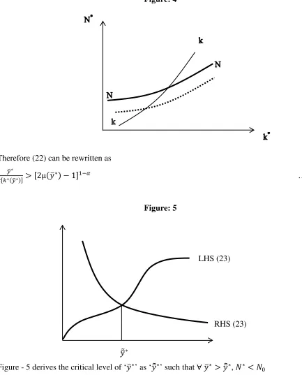
This defines kk in figure-4. Similarly, (19) defines NN in figure-4 with ‘k*’ adjusting along kk and ‘N*’ adjusting along NN. An increase in ‘𝑦𝑦�∗’ shifts NN to the right lowering ‘k*’ and ‘N*’.
Figure: 4
Therefore (22) can be rewritten as
𝑦�∗
𝑥[𝑘∗(𝑦�∗)]> [2µ(𝑦𝑦�
∗)−1]1−𝛼 … (23)
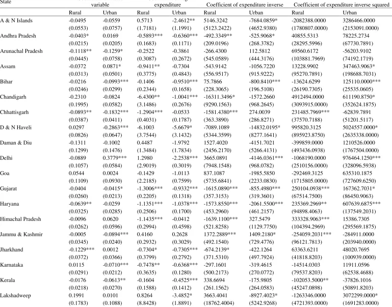
[image:14.612.76.509.143.680.2]Figure: 5
Figure - 5 derives the critical level of ‘𝑦𝑦�∗’ as ‘𝑦𝑦��∗’ such that ∀𝑦𝑦�∗ > 𝑦𝑦��∗, 𝑁∗ <𝑁0
Note that as 𝑦𝑦�∗→0, 𝑁∗ → 𝑥(𝑘∗)
As 𝑦𝑦�∗ → 0 , LHS in (23)→0 and RHS in (23) → a positive value. LHS (23)
RHS (23)
Similarly, as 𝑦𝑦�∗→ ∞LHS will entirely dominate RHS. Thus𝑦𝑦��∗is unique. Thus we can state the following core proposition of the paper.
Proposition 2
If the degree of inequality of income crosses a critical threshold, status concerned
individual will consume less of the nutritious good and may be malnourished even if she
accumulates more than an individual who is not concerned for the relative status.
Proof:
For 𝑦𝑦�∗ ∈(𝑦𝑦��∗,∞), 𝑁∗ <𝑁0, though 𝑘∗ >𝑘0. If 𝑁∗ drops substantially, it may fall below the critical minimum required for nutrition. Q.E.D.
Our paper shows that if people care about social status, they will accumulate more because they value improvement in their relative status. But they cannot avoid a critical substitution effect. Status concerned individual will try to signal their status by consuming more of the status-good and less of the nutritious good. Thus, concern for status will lead to greater accumulation and less nutrition. But that critically depends on the extent of the income effect i.e., 𝑥(𝑘∗)− 𝑥(𝑘0). An increase in𝑦𝑦�∗, the average income of the reference group, will also reduce the rate of accumulation as the marginal utility from status declines with the increase in ‘𝑦𝑦�∗’. However, the level effect will be dominating, meaning𝑘∗ > 𝑘0. If income effect of status is not substantial, nutrition is likely to suffer due to the substitution effect.
Remarks
One implication of the result derived in the paper is relevant for the debate on the conflicting measures of poverty as reported in Patnaik (2007), Marjit (2012), etc. Consider a situation where the representative agent’s income 𝑥(𝑘0) is below poverty line defined in terms of income. If she is concerned about status, she will choose a 𝑘∗ >𝑘0. 𝑥(𝑘∗) >𝑥(𝑘0) indicates an improvement in terms of the poverty measure. In particular if ‘𝑥�’ represents the poverty line, 𝑥(𝑘∗) >𝑥� >
𝑥(𝑘0) means an end of poverty for the agent. However, by the same argument if 𝑁� >𝑁0
of nutrition there will be more people under poverty line. Thus growth with malnutrition will also imply conflicting measures of poverty.
III. Empirical Analysis:
Given the massive impact that distribution of income has on one’s perception of her status in the society and thus her consumption decisions, it becomes vital at this stage to see the impact of such perceptions on one’s decision making process, empirically. As the theory has already established that status concerns have an adverse effect on the nutritional state of the people, even in the face of rising incomes, here we exemplify the existence of such a phenomenon empirically. For our purpose, we take up India, as a prospective candidate and look for the prevalence of status, affecting the relative consumptions of commodities.
In India, it is often observed that higher levels of overall consumption expenditure (which is
approximated as a proxy for income levels) among the poor do not imply higher nutritional intake which is quiet contrary to general perception. World Bank Data reveals, in the past decade, India has seen high annual growth rates from about 4 percent to an average of 8 percent peaking to about 10 percent in 2011. Also the poverty levels (according to World Bank data) have reduced over years. But the nutritional status of many states of the country does not show respectable levels of improvement. Svedberg (2008) found that between 1993 and 2006, net state domestic product per capita grew by about 4.5% per year on an average, nearly a doubling of real income, while the prevalence of child stunting and underweight reduced by a meagre 23 percent to 12 percent over the past 13 years. Whereas in China, child stunting fell from 33 to 10 percent during 1992-2005 and child underweight was practically eliminated. Also prevalence of under nutrition in adult women in 2005-2006 was 33%, down only by 3 percentage points from 36 percent in 1998-19991.
The reason behind such perverse outcomes, have been attributed in our paper to a status effect (the inherent tendency to consume status goods rather than nutritious goods to conform to societal status) prevailing among the population which interacts with the income effect and determines the overall relative consumption patterns. In many middle income countries it has been observed that as the income levels of the people rises, with a rise in income inequality, the low income people try to mimic the consumption pattern of higher income class, thereby
1
International Institute of Population Sciences, Research Brief, No. 2, (2007).
bringing a shift in their expenditure structure toward luxury goods and thus affecting their nutritional status. This would imply another aspect of income inequality – that income inequality distorts consumption and expenditure patterns among the poor. In accordance with the theory developed so far, we consider a situation where the poor people are concerned about their relative social status. In a society with unequal distribution of income, to keep up with the standards of the high income class, low income people try to spend more on luxury goods so as to retain their relative status. In other words, income inequality in a society has an impact on the tendency to retain relative social status among the poor. This can be quantified by the spending on non-food luxury items in comparison to food items.
The following section elucidates the methodology of our analysis and the assumptions of the model used along with the results obtained thus.
IV. Data and Methodology
The entire empirical analysis is entirely based on the extensive dataset provided by the National Sample Survey Organization of India viz. the NSS 66th and 68th round all India unit level survey on consumption expenditure (Schedule1.0, Type 1 and 2). The dataset includes household level observations on item specific expenditure and various household specific characteristics. Apart from this, data is also provided on the households’ localization, such as the sector (Rural or Urban), district and state. The total number of household level observations in our analysis is 201649 for the 66th round and 203313 observations for the 68th round. The data spans thirty five states and union territories. The total number of districts in our analysis is 612 for the 66th round and 625 for the 68th round.
Tables 1a and 1b summarize some of the key statistics related to the principal variables of our analysis namely the monthly per capita expenditure which is further subdivided into monthly per capita expenditures on food and non-food commodities. These statistics are reported for both the rounds and are categorized according to the individual states and sectors as well as for the overall country as a whole. To motivate our empirical model, we first present a preliminary empirical exercise. For a particular round of data, we consider only those households of rural India who’s monthly per – capita consumption expenditures lie within a range2 of 250 rupees above or below the rural India’s lowest quintile (i.e., 25th percentile) level of monthly per – capita consumption
2
Taking into consideration the number of data points available for the analysis and the difference between the upper limit of the range (which is 250 rupees above the quintile) with the median.
expenditure. For these households, we consider their per capita monthly expenditure on food and non – food commodities and compute the district wise average food to non-food expenditure ratios. We plot these figures against the respective districts’ rural median monthly per – capita total consumption expenditure. We redo this exercise separately for urban India considering the per capita monthly expenditure on food and non – food commodities of those households who’s monthly per – capita consumption expenditures lie within the specified range above or below the urban India’s lowest quintile level of monthly per – capita consumption expenditure. From this data, we likewise calculate the district wise average food to non-food expenditure ratios and plot it in a diagram against the respective districts’ urban median monthly per – capita total consumption expenditure. both rounds of the data. The plots from this exercise for both rounds of data are depicted in figure – 6. We find that each of the scatterplots depicts a negative relationship between the district and sector wise average expenditure ratios and the
corresponding district and sector wise median total consumption figures. To illustrate this clearly, we have also, we fitted a linear trend line to each of the scatterplots. These plots are in line with our conjecture and bears out the fact that relatively poor individuals belonging to a particular class of income (here proxied by total consumption expenditure), do tend to “mend their self” by revising their consumption patterns in a way that mimics the consumption patterns of the relatively richer sections in their societies.
With this initial result in hand, we move on develop a detailed and robust statistical framework in the subsequent paragraphs to study the nature and significance of the role of status in shaping individuals’ consumption patterns.
For our formal statistical model, we first need to identify the households who are subject to the aforementioned status concerns. So, we consider each hamlet–group/sub–block of every first stage sampling units (FSU)3 and admit into our analysis only those households whose monthly per capita consumption expenditures (which serves as a proxy to the respective household’s per capita income) lie below the hamlet–group’s/sub–block’s median per capita consumption expenditure level.
3
These FSU’s are the 2001 census villages (Panchayat wards in case of Kerala) in the rural sector and Urban Frame Survey (UFS) blocks in the urban sector. In addition, for the 66th round, two towns of Leh and Kargil of Jammu & Kashmir are also treated as FSUs in the urban sector. These FSUs are further subdivided into hamlet–groups for rural sector and sub–blocks for urban sector, in case the population of a FSU is found to be more than a certain threshold (1200 for most cases and 600 for other areas), more or less equalizing the population in each hamlet– groups/sub–blocks.
Next, in order to define a status variable for these households, we take up every prospective household satisfying the above criterion and for each of these household, consider those households which reside in the same hamlet–group/sub–block but having per capita consumption expenditures above the hamlet–group’s/sub–block’s highest quintile (i.e., 75th percentile) and take the logarithm of their median per capita consumption expenditure as the status variable of the prospective household. The status variable constructed thus, also makes our analysis robust to specification biases. This follows since the manner in which the status variable of a household is defined makes it irresponsive to the household’s income up to a certain extent thus guarantying that this variable truly represents the households’ responsiveness to its societal position rather than capturing certain nonlinearity of the households’ income.
Next, we divide the consumables into two categories: food, and non-food and consider the ratio of food to non-food expenditure. To test for the presence of status concern of the selected
households, we look at the relationship of their expenditure share on income level (proxied by per capita expenditure), the status variable and a few other covariates which act as controls. Our underlying theoretical model to this empirical exercise assumes that the ratio of expenditure on food to non-food has a multiplicative relationship with income and status, which is given by:
𝑆=�𝐸𝑓
𝐸𝑛𝑓�=𝐺1(𝑝)𝐺2(𝑀)𝐺3(𝐷)𝐺4(𝑍)ℇ
In the above relation, E represents the total expenditure on the subscripted commodity which may be food (f), or non-food (nf), p denotes the vector of prices of the consumables, 𝐺𝑖(∙)∀𝑖= 1 to 4 are arbitrary functions, M, D denote income and the status variable respectively, Z
represents a vector of other control variables and ℇ represents a log-normal error term. Taking natural logarithm of the above equation, we get a log linear relationship as:
ln𝑆=𝐹1(𝑝) +𝐹2(𝑀) +𝐹3(𝐷) +𝐹4(𝑍) +𝜀
… (24) where 𝐹𝑖(∙) ≡ ln𝐺𝑖(∙)∀𝑖= 1 to 4
Note that our previous assumptions on the error component imply that 𝜀 follows a normal distribution with mean zero and some variance.
We estimate equation (24) with some additional structure particularly on the functional forms of
𝐹𝑖(∙)′𝑠 as well as on the error term. Specifically we estimate the system:
ln𝑆𝑖𝑗 = 𝛼𝛼𝑖 +𝛽𝑖ln𝑀𝑖𝑗 +𝛾𝑖 1
𝑀𝑖𝑗+𝛿𝑖
1
where 𝜀𝑖𝑗|𝑀𝑖𝑗,𝐷𝑖𝑗,𝑍𝑖𝑗~𝑁(0,𝜇𝜇𝑖2) , the subscript ‘i’ indexes the possible combinations of states and sectors while ‘j’ indexes the households belonging to the particular combination of state and sector indexed by ‘i’.
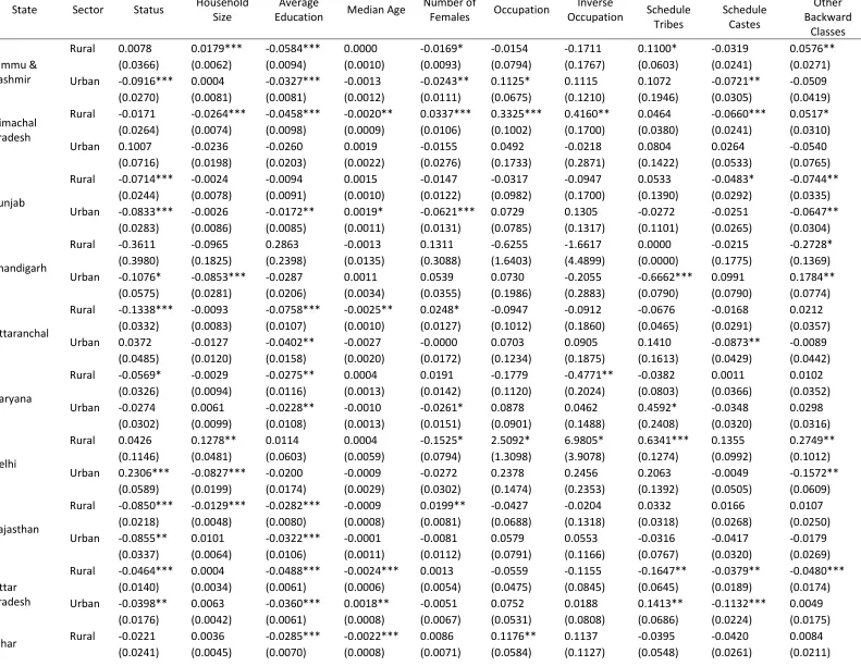
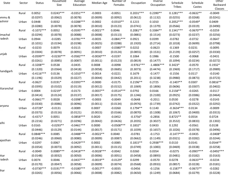
In the above equation, the state-sector specific intercept term:𝛼𝛼𝑖 not only takes care of the functional dependence of the consumption share with the prices which are assumed to be invariant within any the state-sector ‘i’, but also includes any other state-sector specific “fixed effects” that may be correlated with the other exogenous variables. Also the coefficients associated with both the status variable and the different functional forms of income, are allowed to vary across the states and sectors so as to permit changes in the patterns of consumption across the different states and sectors of India. For the control variables, we have incorporated a number of household specific characteristics that include: the household size, the average level of education4, the median age, the number of females, the principal occupation class5, the inverse of the principal occupation class, and indicators for the social group6. The above system is estimated using generalized least squares. The results of this empirical exercise are elucidated next.
V. Results and Discussion
If poor people are indeed concerned about their relative standing in the society then it must get
reflected in our empirical exercise as a significant𝜃𝑖: the coefficient associated with the log of the variable indicating status effect. If 𝜃𝑖 is significantly negative, it indicates that for the particular state and sector indexed by ‘i’, a rise in income inequality coerces the individuals who are relatively poor, to consume food commodities in relatively lesser quantities compared to other non-food items.
The results estimated NSS 66th round data reveals that status effect among the poor affects more or less symmetrically both the urban and rural sectors of the different states of India. For the urban sector, out of the thirty five states (henceforth, the union territories will be referred to
4
The general educational level of an individual is indicated by numbers where – not literate: 0, literate without formal schooling: 1, literate with formal schooling below primary: 2, primary: 3, middle: 4, secondary: 5, higher secondary: 6, diploma/certificate course: 7, graduate: 8, postgraduate and above: 9.
5
The principal occupations are divided into the following categories – legislators, senior officials and managers: 1, professionals: 2, technicians and associate professionals: 3, clerks: 4, service workers and shop & market sales workers: 5, skilled agricultural and fishery workers: 6, craft and related trades workers: 7, plant and machine operators and assemblers: 8, elementary occupations: 9, new workers seeking employment or workers reporting occupations unidentifiable or workers not reporting any occupations: 10.
as states) considered, the estimated coefficient of 𝜃 is significantly negative in fifteen states. The coefficient of the status variable assumes a statistically significant negative value for the states of Gujarat, Uttar Pradesh, Kerala, Karnataka, Rajasthan, West Bengal, Jammu & Kashmir, Punjab, Bihar, Tamil Nadu, Madhya Pradesh, Arunachal Pradesh, Tripura, Chhattisgarh and D & N Haveli, arranged in terms of increasing absolute value of the said coefficients. [Refer Table: 2a]
For the rural sector, a negative significant coefficient of the status variable has been registered for a total of sixteen out of the thirty five states. The coefficient of the status variable assumes a statistically significant negative value for the states of Maharashtra, Andhra Pradesh, Uttar Pradesh, Madhya Pradesh, Punjab, Haryana, Tamil Nadu, Orissa, Rajasthan, Chhattisgarh, Sikkim, Arunachal Pradesh, Jharkhand, Uttaranchal, Meghalaya and Mizoram, arranged in terms of increasing absolute value of the said coefficients. [Refer Table – 2a].
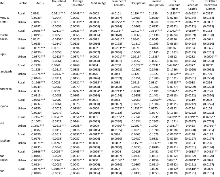
Similarly, using the 68th round data, we find that, for the urban sector, the coefficient of the status variable associated with the fourteen states have assumed a significantly negative value. These states are Madhya Pradesh, Maharashtra, Punjab, Bihar, Assam, Tamil Nadu, West Bengal, Gujarat, A & N Islands, Pondicherry, Mizoram, Tripura and Chandigarh arranged in terms of increasing absolute value of the said coefficient. For the rural sector, the coefficients of the status variable for the states of West Bengal, Maharashtra, Bihar, Haryana, Karnataka, Madhya Pradesh, Tripura, Gujarat, Chhattisgarh, Himachal Pradesh, Manipur, Assam and
Chandigarh arranged in a similar manner, have assumed a significantly negative value. [Refer Table – 2b].
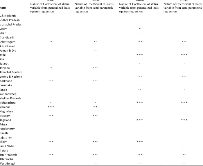
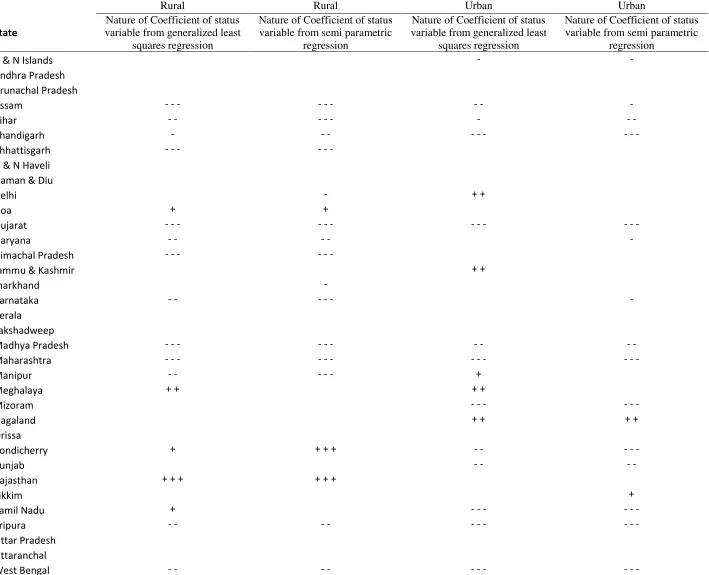
VI. Robustness
In order to further our claims, we forward some additional results that serve as a check for robustness of the relationship between the relative food to non-food consumption share and the status variable. For this purpose, we repeat the above exercise using a semi parametric regression techniques as suggested by Robinson (1988) and checked the variation in our finding. In this alternate formulation, we do not assume any functional form of the association of income with the relative consumption share and estimate the relationship: ln𝑆=𝛼𝛼+
𝐹(𝑀) +𝜃ln𝐷 +𝜌𝑍+𝜀, for each possible combination of state and sector separately. The
6
The social groups are – social group : Scheduled Tribes: 1, Scheduled Castes: 2, Other Backward Classes: 3 and the rest: 9.
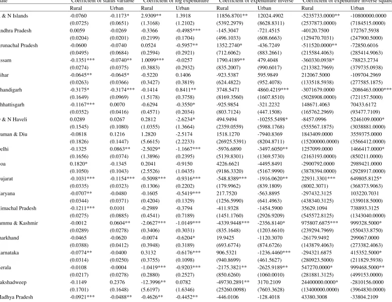
results from this new exercise are summarized in tables 3a and 3b. If we consider only the significance and the sign of the coefficients associated with the status variable and compare the estimates obtained from the semi parametric regression with our previous estimates from the generalized least squares regression, we observe some discrepancies for the states of Arunachal Pradesh, Chandigarh, Daman & Diu, Madhya Pradesh, Tripura and West Bengal using 66th round data and for Delhi, Jharkhand and Andaman and Nicobar Islands using that of 68th Round data. However for a majority of the combinations of states and sectors, the two regression techniques seem to tally both in terms of the sign and significance of the estimated coefficients [Refer Table – 4a and b].
Since for the semi parametric model, we have run our regression separately for every combination of the states and the sectors, we conduct another exercise where we have pooled the data from both the rounds and estimate the semi parametric model separately for both the
states and introduce a time dummy with the intercept term to account for the intertemporal changes in prices as well as other factors which may be correlated with the exogenous variables. This approach increases the number of observations available for the regressions and thus provides us a better estimate of the model parameters as well as the associated standard errors. The result from this final analysis is illustrated in table 5. The figures indicate that for this pooled regression, the coefficient of the status variable assumes a significant negative value for a majority of thirty eight – out of the possible seventy possible combinations of states and sectors. Arranged in increasing absolute magnitude of the coefficient associated with the status variable, these combinations are the rural sectors of the states: Uttar Pradesh, Bihar, Karnataka, West Bengal, Orissa, Punjab, Maharashtra, Himachal Pradesh, Gujarat, Haryana, Madhya Pradesh, Tripura, Sikkim, Assam, Arunachal Pradesh, Chhattisgarh, Jharkhand, Meghalaya, Uttaranchal, Mizoram and Delhi, and the urban sectors of the states: Uttar Pradesh, Kerala, Rajasthan, Gujarat, Karnataka, Chhattisgarh, Madhya Pradesh, Punjab, Arunachal Pradesh, West Bengal, Tamil Nadu, Bihar, A & N Islands, Chandigarh, Mizoram, Tripura and D & N Haveli.
VII. Conclusion
In this paper we wanted to focus on the impact of relative status on the consumption behaviour of the poor who might feel relatively deprived in a society with highly unequal income distribution. We have demonstrated that concern for social status in a situation where a rise individual income is also accompanied by a worsening of income distribution, people may spend less on food and more on status good. Thus income based and nutrition-based measures of poverty will give qualitatively different result and income growth will be consistent with malnutrition. After theoretical demonstration we test our results in terms of the NSSO 66th and 68th round datasets across Indian states and estimation through various methodologies strongly corroborate our claim. In many states we cannot rule out the negative impact of inequality, which is the key force behind the concern for status, on relative consumption of food. Future work will try to explore the implication of such concern for status on health, education and
gender related issues.
References
Banerjee, A. V., & Duflo, E. (2011). Poor Economics: A Radical Rethinking of the Way to Fight Global Poverty. New York: PublicAffairs.
Beath, J., & Fitzroy, F. (2010). Status, Hapiness and Relative Income. IZA Discussion Paper No. 2658 .
Clark, A. E., & Oswald, A. J. (1996). Satisfaction and Comparison Income. Journal of Public Economics, LXI, 359–381.
Cole, H. L., Mailath, G. J., & Postlewaite, A. (1992). Social Norms, Savings Behavior, and Growth. Journal of Political Economy, Vol. 100(6), 1092-1125.
Corneo, G., & Jeanne, O. (2001). Status, the Distribution of Wealth, and Growth. Scandinavian Journal of Economics, Vol. 103(2), 283-293.
Deaton, A., & Dreze, J. (2009). Food and Nutrition in India:Facts and interpretation. Economic & Political Weekly, 44(7), 42-65.
Easterlin, R. A. (1974). Does Economic Growth Improve the Human Lot? Some Empirical Evidence. In P. A. David, & M. W. Reder, Nations and Households in Economic Growth: Essays in Honor of Moses Abramowitz. New York: NY: Academic Press.
Easterlin, R. A. (1995). Will Raising the Incomes of All Increase the Happiness of All? Journal of Economic Behavior and Organization, XXVII, 35–48.
Easterlin, R. A. (2001). Income and Happiness: Towards a Unified Theory. Economic Journal, CXI, 465–484.
Fafchamps, M., & Shilpi, F. (2008). Subjective welfare, isolation, and relative consumption.
Journal of Development Economics, Vol. 86(1), 43-60.
Ferrer-i-Carbonell, A. (2005). Income and Well-Being: An Empirical Analysis of the Comparison Income Effect. Journal of Public Economics, LXXXIX, 997–1019.
Frank, R. H. (1985). The Demand for Unobservable and Other Nonpositional Goods. American
Economic Review, Vol. 75(No. 1), 101-116.
Ghiglino, C., & Goyal, S. (2008). Keeping up with the neighbors: social interaction in a market economy. ournal of the European Economic Association, 8(1), 90-119.
Government of India. (2011-12). Economic Survey.
Griffiths, P., & Bentley, M. (2001). 'The Dual Burden of Nutrition Transition for Women in India:A Comparision of the Rural Poor and Urban Elite in Andhra Pradesh'. The Journal of Nutrition, 131(10), 2692-2700.
Heltberg, R. (2009). Malnutrition, poverty, and economic growth. Health Economics, Vol.18(1). Hopkins, E., & Kornienko, T. (2010). Which Inequality? The Inequality of Endowments Versus
the Inequality of Rewards. American Economic Journal: Microeconomics, 2(3), 106-137. Kanbur, R., & Tuomala, M. (2010). Relativity, Inequality and Optimal Nonlinear Income
Taxation. Working Paper, Cornell University.
Ku, H., & Salmon, T. C. (2009). Incentive Effects of Inequality and Economic Development.
Mimeo, Florida State University.
Luttmer, E. F. (2005). Neighbors as Negatives: Relative Earnings and Well Beings. Quarterly Journal of Economics, Vol. 120(3), 963-1002.
Marjit, S. (2012). Conflicting Measures of Poverty and Inadequate Saving by the Poor. Working Papers UNU-WIDER Research Paper , World Institute for Development Economic
Marjit, S., & Roychowdhury, P. (2012). Inequality, status effects and trade. MPRA Paper 40225, University Library of Munich, Germany.
McBride, M. (2001). Relative-Income Effects on Subjective Well-Being in the Cross-Section.
Journal of Economic Behavior and Organization, XLV, 251–278.
Moav, O., & Neeman, Z. (2012). Saving Rates and Poverty: The Role of Conspicuous Consumption and Human Capital. The Economic Journal, 122(563), 933-956.
Mujcic, R., & Frijters, P. (2013). Economic choices and status: measuring preferences for income rank. Oxford Economic Papers, 65(1), 47-73.
Mukherjee, A., Rajaraman, D., & Swaminathan, H. (2010). Economic Development, Inequality and Malnutrition in India. IIM Bangalore Working Paper.
Patnaik, U. (2007). Neoliberalism and Rural Poverty in India. Economic and Political, Vol.
42(30), 3132-3150.
Radhakrishna, R., & Ravi, C. (2004). Malnutrition in India: Trends and Determinants. Economic and Political Weekly, 30(7), 671-676.
Ray, D., & Robson, A. (2012). Status, Intertemporal Choice, and Risk-Taking. Econometrica, Vol. 80(4), 1505-1531.
Robinson, P. M. (1988). Root-n-consistent semiparametric regression. Econometrica, vol. 56, 931-954.
Robson, A. (1992). Status, the Distribution of Wealth, Private and Social Attitudes to Risk.
Econometrica, Vol. 60(4), 837-857.
Senik, C. (2004). Relativizing Relative Income. Manuscript, DELTA and University Paris-IV Sorbonne.
Sivanathan, N., & Petit, N. (2010). Protecting the self through consumption of Status goods.
Journal of Experimental Social Psychology, Vol. 46, 1238-1244.
Svedberg, P. (2008). Why Malnutrition in Shining India Persists. 4th Annual Conference on Economic Growth and Development. ISI Delhi.
Van de Stadt, H., Kapteyn, A., & Van de Geer, S. (1985). The Relativity of Utility: Evidence from Panel Data. Review of Economics and Statistics, LXVII, 179-187.
Veblen, T. (1902). The Theory of the Leisure Class: An Economic Study of Institutions. New York: Macmillan.
Table 1a: Descriptive statistics of important variables for the 66th round.
Monthly Per Capita Expenditure Monthly Per Capita Food Expenditure Monthly Per Capita Non Food Expenditure
State Sector Mean Median SD Min Max Obs Mean Median SD Min Max Obs Mean Median SD Min Max Obs
Jammu & Kashmir
Rural 1362.39 1203.615 693.0399 322.6367 16502.92 2891 732.903 658.6 298.9507 204.875 3845.905 2891 629.4866 513.726 503.2903 100.126 15060.54 2891
Urban 2302.122 1874.22 1817.317 452.1689 30792.03 2537 895.3167 793.75 424.453 239 7730 2537 1406.806 1045.896 1559.882 101.863 28388.69 2537
Himachal Pradesh
Rural 1680.269 1352.732 1263.977 284.3021 26695.75 3320 810.1229 700.9429 427.0145 168.1667 7038.714 3320 870.1463 614.2876 982.7139 38.3351 23942.25 3320
Urban 3424.801 2767.948 3599.817 424.8 64588.27 763 1218.754 1058.952 854.5211 194.6 9869.286 763 2206.047 1561.575 3093.607 135.1712 63200.27 763
Punjab Rural 1751.492 1395.967 1555.849 284.5531 33246.46 3118 803.8595 704.8979 372.0106 202.875 7170.4 3118 947.6323 664.4247 1341.18 81.6781 30845.13 3118
Urban 2688.532 2113.383 2071.322 302.637 19208.16 3112 966.3746 840 516.0335 211 6921.429 3112 1722.157 1159.151 1737.054 91.637 15578.84 3112
Chandigarh Rural 2691.761 2162.486 1533.186 745.2485 8755.73 64 1037.541 897.25 457.9251 361.2 2803.857 64 1654.22 1294.808 1359.853 274.8676 7820.73 64
Urban 5284.247 4183.067 4390.18 473.9076 30621.43 546 1506.175 1175 1126.848 270.75 12200.71 546 3778.072 2572.836 3772.854 133.3233 28184.43 546
Uttaranchal Rural Urban 3355.443 2407.37 1296.228 1933.932 3988.326 1597.498 337.8755 301.1693 13447.49 16147.32 1461 2093 877.234 1132.219 779 698.7143 909.7914 430.8543 198.5 150 4050.143 4765.5 1461 2093 1530.136 2223.224 1103.115 549.6458 1281.398 3105.423 141.0771 73.3534 14834.68 10441.49 2093 1461
Haryana Rural 1543.384 1302.072 940.2314 301.7363 16574.85 2880 801.4947 730.2321 425.4056 149.3214 8611.393 2880 741.8896 559.1096 632.3874 89.4658 14672.65 2880
Urban 2935.598 2018.437 2896.279 366.1866 28711.91 2360 996.0188 855.5714 628.5407 190.4 6414.572 2360 1939.579 1174.233 2388.878 90.7945 22297.34 2360
Delhi Rural 2181.344 2076.315 1205.339 727.2192 7625.231 116 1166.063 984.6667 840.7632 362.8 5644.286 116 1015.281 863 468.0908 364.4192 3124.793 116
Urban 3746.306 2760.288 2972.32 456.8853 25034.91 1650 1154.699 1046.143 613.7545 200.625 8993 1650 2591.607 1680.041 2568.224 210.9178 23505.91 1650
Rajasthan Rural 1196.387 1024.861 957.7786 242.1204 19826.24 5158 639.3392 578.1905 384.8109 119.6429 13547.76 5158 557.0481 435.2123 639.9851 75.1747 11409 5158
Urban 2298.979 1759.407 1808.895 340.6082 21347.92 3104 854.3326 736.3333 517.6811 163.8333 10557.14 3104 1444.647 999.7466 1432.303 135.4794 19775.92 3104
Uttar Pradesh Rural 939.2199 805.0366 575.3915 159.7123 22050.46 11814 526.5634 467.1714 294.6266 42.8571 14295.64 11814 412.6565 323.674 363.2023 27 20099.1 11814
Urban 2545.087 1534.681 3161.204 285.2466 22581.55 6173 838.0306 638.25 637.0249 136.6667 12857.14 6173 1707.056 860.9543 2654.558 99.4857 20823.05 6173
Bihar Rural 797.2713 712.7292 371.0808 154.5744 9659.173 6593 495.0195 453.2727 212.5169 110.4 3007.5 6593 302.2518 253.7489 199.2145 20.6849 8968.459 6593
Urban 1602.362 1257.496 1183.492 158.2123 11176.36 2542 699.3577 579.3214 404.792 98.6667 3985 2542 903.0041 645.0607 873.7448 8.7123 8920.356 2542
Sikkim Rural 1609.14 1165.521 1440.506 425.1308 18170.63 1216 789.4375 635.8333 613.3556 267.6286 17057.14 1216 819.7029 547.863 931.0383 120.0593 8352.261 1216
Urban 2741.348 2384.843 1691.175 576.5753 18120.86 320 1182.327 1015.25 574.5399 393.6 2950 320 1559.02 1171.84 1351.699 76.5753 16094.36 320
Arunachal Pradesh
Rural 1591.304 1231.411 1134.765 297.7973 11843.18 2082 860.5166 678.9286 640.9535 173 8471.536 2082 730.7878 525.3699 626.168 34.4 8922.329 2082
Urban 2001.265 1649.848 1374.548 228.3105 15139.74 1200 946.8739 793.1429 631.6078 134 7208.429 1200 1054.391 803.4058 906.5038 81.6438 11202.74 1200
Nagaland Rural 1491.478 1357.059 601.8869 592.1592 7612.288 1408 826.0288 771.2571 281.5772 397.5714 6000 1408 665.4494 558.8983 410.6178 112.1592 4317.842 1408
Urban 2148.858 1930.948 1054.102 781.613 13158.55 640 904.8238 801.7143 384.8495 353.8571 2828.572 640 1244.034 1062.705 774.6839 265.9501 10646.91 640
Manipur Rural 1011.958 937.2466 361.0962 436.6446 6081.137 2752 589.3497 560.1667 160.9309 233 2124.714 2752 422.6084 374.3059 259.5195 107.7652 5394.887 2752
Urban 1404.212 1183.905 750.9621 520.0106 12128.49 2364 609.9689 552.25 328.3592 231.125 11619.37 2364 794.2434 641.7432 559.3308 50 7864.859 2364
Mizoram Rural 1239.616 1110.112 567.3801 394.6931 5785.71 1264 706.4235 655.0476 288.2805 219.25 2933.286 1264 533.1926 458.8155 341.677 108.8359 3532.293 1264
Urban 2229.578 2048.221 1068.317 470.2082 13219.92 1792 972.7754 898 437.1347 174.2 4120.334 1792 1256.802 1098.822 716.9358 234.683 12227.82 1792
Tripura Rural 1132.345 1021.021 526.6854 340.9139 7181.109 2623 700.9773 638 281.0407 192.4 3379.714 2623 431.3676 356.2123 302.1563 77.5703 5108.609 2623
Urban 2205.532 1841.294 1473.515 409.1507 11349.41 1088 997.2024 895.6428 486.914 182.5 3817.714 1088 1208.33 897.5822 1087.149 88.2054 9396.411 1088
Meghalaya Rural 1121.695 998.6693 470.5018 392.1811 7131.536 1728 606.5406 545.0357 233.6059 201 3713.143 1728 515.1544 444.5856 294.4006 135.9949 5324.679 1728
Urban 1980.296 1716.9 1112.081 498.8995 12517.84 816 744.4296 654.4 332.0241 235.0357 4031 816 1235.867 983.9384 863.7781 230.2003 8486.836 816
Assam Rural 975.4923 862.5362 461.7016 309.9486 7842.81 5232 625.0082 574.4081 254.3916 154.25 3103.679 5232 350.4841 276.2505 271.8193 46.0137 7084.953 5232
Urban 2140.483 1790.307 1485.003 391.9699 34953.06 1664 954.9719 822 510.6677 200 3387 1664 1185.511 855.5494 1083.494 62.6274 32282.42 1664
West Bengal Rural 962.1634 859.2707 509.6894 232.0959 26210.04 7151 581.8862 534.9429 266.6622 105.4 12712.43 7151 380.2772 307.7306 306.7618 39.1986 13497.61 7151
Urban 2562.613 1806.685 2501.527 108.2818 32076.29 5499 925.5439 784.5 578.9654 74.3571 13563.5 5499 1637.069 937.2856 2122.752 33.9247 25793.81 5499
Jharkhand Rural 821.4512 721.1924 373.148 182.4384 11282.94 3516 485.4108 436.75 211.7506 106.8571 2900.786 3516 336.0404 273.7432 208.6291 49.5863 8382.152 3516
Urban 1915.1 1440.082 1610.707 277.0255 14451.12 1979 831.4848 675.8095 554.7258 154.7143 7021.571 1979 1083.615 719.5671 1171.931 81.0548 11677.12 1979
Orissa Rural 821.7712 699.6678 497.535 87.5616 24083.93 5949 494.6487 432.1429 280.0689 20 3440.048 5948 327.7208 258.6927 285.9688 50 22940.85 5948
Urban 2062.45 1497.792 1992.382 271.0455 21017.19 2110 803.5914 666.2857 527.2601 31.4 4951 2110 1258.859 772.4384 1655.497 85.0941 18413.19 2110
Chhattisgarh Rural 786.3967 670.6986 442.2205 151.4286 5970.54 2991 431.3263 389.6 219.3563 20 2849.143 2991 355.0704 286.6165 274.9353 0 4730.534 2991
Urban 1951.639 1550.77 1523.911 207.1918 21928.26 1472 702.233 641.3143 377.8328 65.75 7350 1469 1253.027 891.9588 1268.965 0 14578.26 1469
Madhya Pradesh
Rural 917.3286 755.8699 621.6084 165.3892 19509 5465 491.8507 423.0286 290.2208 59.3333 3336 5465 425.4779 323.8995 387.6866 58.0043 18708.6 5465
Urban 2299.18 1593.406 2170.445 305.4521 23304.39 3939 747.9272 617.9841 511.8811 129.6 9047.143 3939 1551.253 958.5114 1755.719 110.7854 21593.58 3939
Gujarat Rural 1178.172 1003.961 909.0963 273.5993 40802.64 3439 643.5385 583.5 263.8387 159.75 2647 3439 534.6339 396.3653 751.6698 77.047 38675.98 3439
Urban 2685.56 2129.617 2147.52 340.532 32428.48 3403 928.3275 851.3333 481.648 118 7152.75 3403 1757.232 1231.113 1858.752 102.8653 30657.48 3403
Daman & Diu Rural 1774.689 1665.154 862.2904 413.1678 7396.447 128 806.1663 814.9286 292.0942 214.875 2128.667 128 968.5228 860.8127 603.4626 198.2928 5267.781 128
Urban 2561.365 1913.137 1620.977 730.1849 9243.193 128 928.5345 792.5 441.524 313.8571 2730.714 128 1632.831 1207.685 1238.246 308.2877 6575.021 128
D & N Haveli Rural 934.8202 768.7531 470.866 410.3151 3032.912 192 579.8487 534.1667 218.1349 228.3333 1707.286 192 354.9714 265.0039 276.9481 109.6205 1649.555 192
Urban 2156.64 1819.926 1236.517 783.9095 8155.2 192 865.6344 780.6285 344.8528 422.5 2368.5 192 1291.006 1013.699 951.9344 305.227 6473.676 192
Maharashtra Rural 1173.623 1040.14 663.9337 95.589 29279.17 8027 612.5145 566.1786 273.3141 92.9643 12607.86 8026 561.6456 442.6439 499.6414 50 23579.06 8026
Urban 3655.821 2347.999 4454.102 268.024 89253.33 7964 1063.719 884.5 665.3053 160.375 8101.714 7962 2592.352 1360.185 4041.76 109.2055 86690.33 7962
Andhra Pradesh Rural 1316.319 1046.507 1065.868 42.1507 27063.9 7852 725.2746 602.1429 487.547 8 5677.143 7847 591.277 416.8174 651.1203 30.0959 23983.75 7847
Urban 2765.193 2066.784 2364.083 287.1233 27492.62 5915 1054.046 846.6786 877.8003 30 17700 5913 1711.257 1132.262 1775.298 57.7397 21826.85 5913
Karnataka Rural 1017.591 874.0068 568.3782 275.2913 9250.538 4074 559.8203 502.7857 250.7264 124.1333 4129.5 4074 457.7704 359.0803 394.2891 65.6233 8104.872 4074
Urban 2864.236 2121.696 2843.924 298.9589 45520.63 4071 948.4206 824.2449 533.5428 15 5991.428 4070 1916.313 1241.368 2524.229 73.2466 44306.63 4070
Goa Rural 2029.313 1817.731 958.2671 657.2945 18045.25 319 1036.284 960.6667 409.1132 373.8571 3934 319 993.0285 807.6082 673.4141 232.2945 15746.25 319
Urban 3452.81 2914.993 2027.396 598.637 15908.81 572 1194.915 1049.333 654.9139 292.7857 5962.5 572 2257.895 1838.589 1519.846 221.7808 13979.52 572
Lakshadweep Rural 2209.208 1673.553 1985.022 612.6787 16381.15 110 1154.979 958.1429 602.0364 399.4667 3458.571 110 1054.229 601.3015 1635.067 189.3253 14179.15 110
Urban 2998.617 2413.146 1849.072 671.7417 14597.5 256 1352.941 1140 696.0636 363.8095 4500 256 1645.676 1182.055 1411.701 183.7417 10951.5 256
Kerala Rural Urban 2035.67 3328.5 1520.726 2366.491 2086.246 4062.314 217.4794 156.7397 83040.92 185855.6 3691 5212 1036.214 862.0216 868.4286 732.3571 571.2995 798.5854 55 30 10041.25 12599.33 3685 5207 2294.586 1175.762 1404.302 730.8202 3604.496 1787.098 133.1765 16.0274 183683.5 80948.21 5207 3685
Tamil Nadu Rural 1187.503 983.9374 860.151 12.774 14689.63 6639 614.5293 552.75 305.3833 38 4506.334 6636 573.6627 413.9771 664.2551 74.1233 13807.84 6636
Urban 2347.064 1818.411 1853.466 323.2479 37693.03 6638 881.7344 754.2857 508.3953 40 6771.429 6635 1465.392 1015.427 1528.064 105.0753 35845.53 6635
Pondicherry Rural 1697.428 1477.928 855.3396 495.8734 10104.84 256 860.6832 774 319.7012 270.4898 3101.572 256 836.7449 670.927 641.0507 198.7808 7648.506 256
Urban 3939.09 2605.39 9326.49 499.4109 108546.7 896 1210.132 1072.238 633.0971 235.3571 5283.714 896 2728.958 1435.617 9166.761 79.5342 106555.5 896
A & N Islands Rural 2225.682 1663.523 2715.139 619.6674 30073.03 544 1120.694 999.5 601.1774 398.5714 8738.571 544 1104.988 640.9589 2423.701 122.0548 27157.03 544
Urban 3484.745 2841.718 2640.828 927.8184 28258.58 576 1341.732 1208.571 631.4319 325.8571 11444 576 2143.014 1509.84 2307.85 314.789 25629.77 576