Munich Personal RePEc Archive
Long memory in the ukrainian stock
market and financial crises
Maria Caporale, Guglielmo and Gil-Alana, Luis and Plastun,
Alex and Makarenko, Inna
Brunel University, London, CESifo and DIW Berlin, University of
Navarra, Ukrainian academy of banking, Ukrainian academy of
banking
October 2013
Online at
https://mpra.ub.uni-muenchen.de/59061/
LONG MEMORY IN THE UKRAINIAN STOCK MARKET
AND FINANCIAL CRISES
Guglielmo Maria Caporale
*Brunel University, London, CESifo and DIW Berlin
Luis Gil-Alana
**University of Navarra
Alex Plastun
Ukrainian Academy of Banking
Inna Makarenko
Ukrainian Academy of Banking
October 2013
Abstract
This paper examines persistence in the Ukrainian stock market during the
recent financial crisis. Using two different long memory approaches (R/S
analysis and fractional integration) we show that this market is inefficient
and the degree of persistence is not the same in different stages of the
financial crisis. Therefore trading strategies might have to be modified. We
also show that data smoothing is not advisable in the context of R/S
analysis.
Keywords:
Persistence, Long Memory, R/S Analysis, Fractional
Integration
JEL Classification:
C22, G12
*
Corresponding author. Department of Economics and Finance, Brunel
University, London, UB8 3PH.
Email: Guglielmo-Maria.Caporale@brunel.ac.uk
**
1. INTRODUCTION
As a result of the recent financial crisis the relevance of traditional models based on the
efficient market hypothesis (EMH) has been questioned. An alternative paradigm is the
so-called fractal market hypothesis (FMH – see Mandelbrot, 1972, and Peters, 1994),
according to which stock prices are not linear and the normal distribution (a basic
assumption of the EMH) cannot be used to explain their movements given the presence
of “fat tails”. Within this framework one of the key characteristics of financial time
series is their persistence or long memory.
This paper uses two different approaches (i.e. R/S analysis and fractional
integration) to estimate persistence in the Ukrainian stock market. In particular, we
show that this feature is not the same at different stages of the financial crisis of
2007-2009. We also show that data smoothing does not improve the R/S method.
The layout of the paper is the following. Section 2 describes the data and
outlines the Hurst exponent method as well as the I(d) techniques used. Section 3
presents the empirical results. Section 4 provides some concluding remarks.
2. DATA AND METHODOLOGY
The R/S method was originally applied by Hurst (1951) in hydrological research and
improved by Mandelbrot (1972), Peters (1991, 1994) and others analysing the fractal
nature of financial markets. Compared with other approaches it is relatively simple and
suitable for programming as well as visual interpretation.
For each sub-period range R (the difference between the maximum and
minimum index within the sub-period), the standard deviation S and their average ratio
are calculated. The length of the sub-period is increased and the calculation repeated
until the size of the sub-period is equal to that of the original series. As a result, each
applied to these values and a regression is run, obtaining an estimate of the angle of the
regression line. This estimate is a measure of the Hurst exponent, which is an indicator
of market persistence. More details are provided below.
1. We start with a time series of length M and transform it into one of length N =
M - 1 using logs and converting stock prices into stock returns:
) 1 ( ,... 3 , 2 , 1 ,
log 1
t M
Y Y N
t t
i (1)
2. We divide this period into contiguous A sub-periods with length n, so that An
= N, then we identify each sub-period as Ia, given the fact that a = 1, 2, 3. . . , A. Each
element Ia is represented as Nk with k = 1, 2, 3. . . , N. For each Ia with length n the
average ea is defined as:
N , k 1,2,3,...N, а 1,2,3...,А
n 1
e n
1
k k,a
a
(2).
3. Accumulated deviations Xk,a from the average ea for each sub-period Ia are
defined as: ( ) 1 , , a k i a i a
k N e
X
. (3)
The range is defined as the maximum index Xk,a minus the minimum Xk,a, within
each sub-period (Ia):
R
Ia
max(
X
k,a)
min(
X
k,a),
1
k
n
.
(4)4. The standard deviation SIa is calculated for each sub-period Ia:
5 , 0 n 1 k 2 a a , k
Ia ) (N e )
n 1 ( S
. (5)
5. Each range RIa is normalized by dividing by the corresponding SIa. Therefore,
obtained adjacent sub-periods of length n. Thus, the average R/S for length n is defined
as:
A
1
i Ia Ia
n (1A) (R S )
) S R
( . (6)
6. The length n is increased to the next higher level, (M - 1)/n, and must be an
integer number. In this case, we use n-indexes that include the initial and ending points
of the time series, and Steps 1 - 6 are repeated until n = (M - 1)/2.
7. Now we can use least square to estimate the equation log (R / S) = log (c) +
Hlog (n). The angle of the regression line is an estimate of the Hurst exponent H. This
can be defined over the interval [0, 1], and is calculated within the boundaries specified
in Table 1.
[Insert Table 1 about here]
An important step in the R/S analysis is the verification of the results by
calculating the Hurst exponent for randomly mixed data. In theory, these should be a
random time series with a Нurst exponent equal to 0.5. In this paper, we will carry out a
number of additional checks, including:
- Generation of random data;
- Generation of an artificial trend (persistent series);
- Generation of an artificial anti-persistent series.
In order to analyse persistence, in addition to the Hurst exponent and the R/S
analysis we also estimate parametric/semiparametric models based on fractional
integration or I(d) models of the form:
, ... , 1 , 0 t , u x ) L 1
( d t t (9)
where d can be any real value, L is the lag-operator (Lxt = xt-1) and ut is I(0), defined for
positive and finite at the zero frequency. Note that H and d are related through the
equality H = d – 0.5.
In the semiparametric model no specification is assumed for ut, while the
parametric one is fully specified. For the former, the most commonly employed
specification is based on the log-periodogram (see Geweke and Porter-Hudak, GHP,
1983). This method was later extended and improved by many authors including
Künsch (1986), Robinson (1995a), Hurvich and Ray (1995), Velasco (1999a, 2000) and
Shimotsu and Phillips (2002). In this paper, however, we will employ another
semiparametric method: it is essentially a local ‘Whittle estimator’ in the frequency
domain, which uses a band of frequencies that degenerates to zero. The estimator is
implicitly defined by:
, log 1 2 ) ( log min arg ˆ
1
m s s d m d d Cd (10)
, 0 , 2 , ) ( 1 ) ( 1
2
T m T s I m d
C m s
s d s s
where m is a bandwidth parameter, and I(s) is the periodogram of the raw time series,
xt, given by:
, 2 1 ) ( 2 1 T t t s i t
s x e
T
I
and d (-0.5, 0.5). Under finiteness of the fourth moment and other mild conditions,
Robinson (1995b) proved that:
, ) 4 / 1 , 0 ( ) ˆ
(d d N as T
m o d
where do is the true value of d. This estimator is robust to a certain degree of
conditional heteroscedasticity and is more efficient than other more recent
Velasco, 1999b, Velasco and Robinson, 2000; Phillips and Shimotsu, 2004, 2005 and
Abadir et al. (2007).
Estimating d parametrically along with the other model parameters can be done
in the frequency domain or in the time domain. In the former, Sowell (1992) analysed
the exact maximum likelihood estimator of the parameters of the ARFIMA model,
using a recursive procedure that allows a quick evaluation of the likelihood function.
Other parametric methods for estimating d based on the frequency domain were
proposed, among others, by Fox and Taqqu (1986) and Dahlhaus (1989) (see also
Robinson, 1994 and Lobato and Velasco, 2008 for Wald and LM parametric tests based
on the Whittle function).
Two of the main Ukrainian stock market indexes, namely the PFTS and UX
indices respectively, are used for the empirical analysis. The sample period goes from
2001 to 2013 for PFTS and from 2008 to 2013 for UX. For most of the calculations we
used the UX index, which is most frequently used nowadays to analyse the Ukrainian
stock market, since the PFTS series, only starting in 2008, is relatively short. The
different periods considered include that of the inflation "bubble" and market
overheating, which created the preconditions for the crisis in 2007, the peak of the
crisis at the end of 2008 and in the early part of 2009, and its attenuation towards the
end of 2009 and in 2010 (Figure 1).
[Insert Figure 1 about here]
The peak of the crisis is defined on the basis of the dynamics of the CBOE
Volatility Index (VIX), which is calculated from 1993 using the S&P 500 prices of
options in the Chicago Stock Exchange, one of the largest organized trading platforms.
It should be noticed that peaks of market volatility at 89.53 and 81.48 were observed
during the announcement of the bankruptcy of Lehman Brothers and AIG in September
same time the decision to restructure the AIG debt led to better investment expectations
of market participants and to a fall of the VIX index to 39.33 (Figure 2).
Also important is the choice of the interval of the fluctuations to analyse, i.e. 5,
30, 60 minutes, one day, one week, one month. We decided to focus on the 1-day
interval, because higher frequency data generates significant fluctuations of fractals, and
lower frequency data lose their analytical potential.
We incorporate data smoothing into the R/S analysis and test the following
hypothesis: data smoothing (filtration) lowers the level of “noise” in the data and
reduces the influence of abnormal returns; smoothing makes the data closer to the real
state of the market.
We use the following simple methods:
1) Smoothing with moving averages (simple moving average and
weighted moving average with periods 2 and 5);
2) Smoothing with the Irwin criterion.
The analysis is conducted for the Ukrainian stock market index (UX) over the
period 2008-2013. Overall we analysed 1300 daily returns. As a control group we chose
daily closes of UX (unfiltered data) and a set of randomly generated data. The estimates
of the Hurst exponent for the mixed data sets are used as a criterion for the adequacy of
the results.
[Insert Figures 3 – 8 about here]
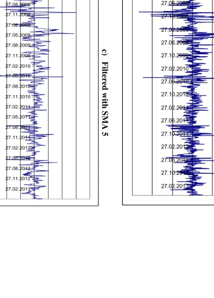
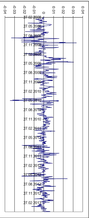
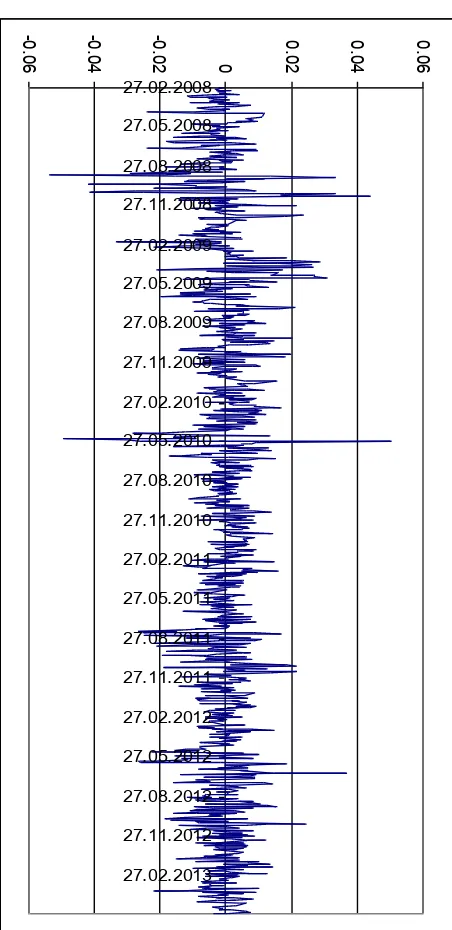
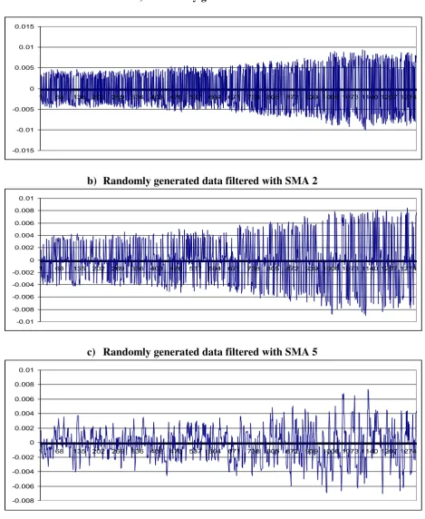
The first stage is the visual analysis of both unfiltered and filtered data. The
results are presented in Figures 3 - 8. The behaviour of the series does not change
dramatically after filtering (smoothing), but the level of “noise” decreases. In terms of
fractal theory, visual inspection reveals a decrease of the fractal dimension.
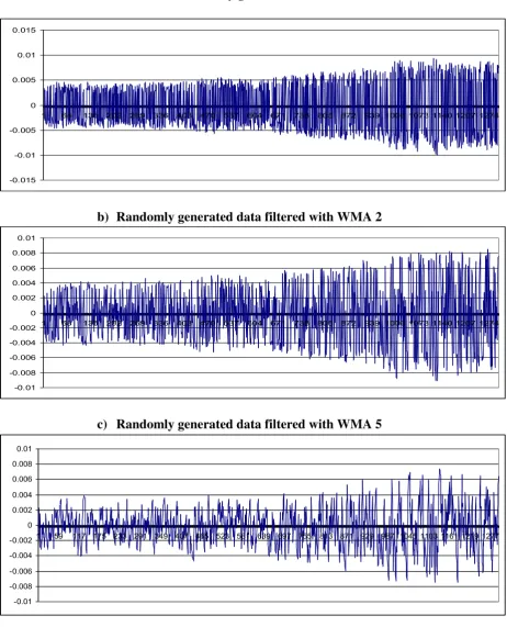
To confirm that the properties of the time series are the same and we only
which the fractal dimension should remain the same. However, visual inspection (see
Figures 6 - 8) shows that the fractal dimension of the randomly generated data set also
changes after filtering.
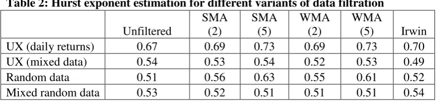
To corroborate the visual analysis we calculate the Hurst exponent for each type
of filter.
[Insert Table 2 about here]
As can be seen from Table 2, filtering the data leads to over-estimating the Hurst
exponent. The longer the averaging period (the bigger the level of filtering) the higher
the Hurst exponent is, indicating dependency of the latter on the former.
Irwin’s method also generates overestimates of the Hurst exponent and therefore
is inappropriate as well. Overall, it appears that data smoothing artificially increases the
Hurst exponent, and therefore further calculations will be based on the original data
sets.
One more possible modification of the R/S analysis is the use of aliquant
numbers of groups, i.e. computing the Hurst exponent for all possible groups. The
results are presented in Table 3.
[Insert Table 3 about here]
Both the real financial data and the randomly generated ones suggest that the use
of aliquant numbers of groups leads to overestimates of the Hurst exponent.
Nevertheless, using them might be appropriate in the case of small data sets, but a
correction of 0.03 - 0.05 should be made depending on the value of the Hurst exponent
(the bigger it is the bigger the correction should be). Given these results, the standard
3. EMPIRICAL RESULTS
As a first stage of the analysis we estimate persistence of two Ukrainian stock market
indices over the full sample (UX: 2008-2013, PFTS: 2001-2013). The results in Table 4
provide evidence of persistence and long memory.
Next, we estimate persistence during the financial crisis. We checked different
window sizes and found that 300 (close to one calendar year) is the most appropriate on
the basis of the behaviour of the Hurst exponent: for narrower windows its volatility
increases dramatically, whilst for wider ones it is almost constant, and therefore the
dynamics are not apparent.
Having calculated the first value of the Hurst exponent (for example, that for the
date 13.07.2007 corresponds to the period from 21.04.2005 till 13.07.2007), each of the
following ones is obtained by shifting forward the “data window”. The chosen size of
the shift is 10, which provides a sufficient number of estimates to analyse the behaviour
of the Hurst exponent. Therefore the second value is calculated for 27.07.2006 and
characterises the market over the period 10.05.2005 till 27.07.2006, and so on. As a
result we obtain 170 control points (Hurst exponent estimates) for different sub-samples
characterised by various degrees of persistence in the Ukrainian stock market over the
period 2005-2013 (see Fig. 9).
[Insert Figure 9 about here]
It is apparent that market persistence is not constant over the sample, increasing
during the crisis. Consequently, trading strategies might have to be revised.
Semiparametric/parametric methods for the UX index
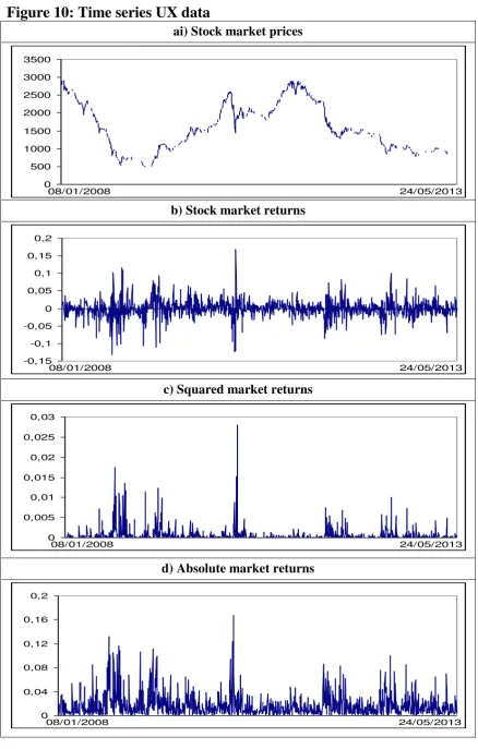
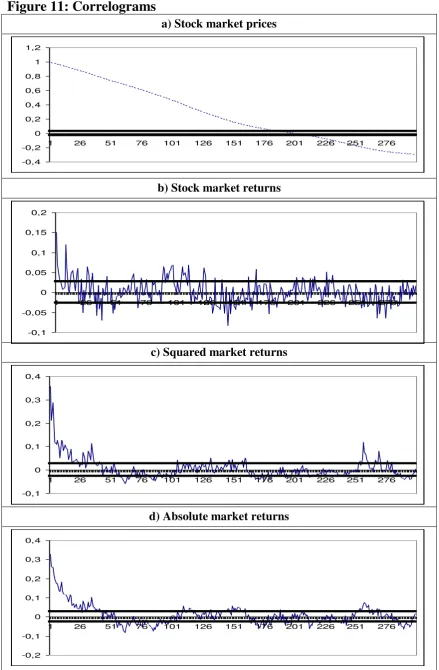
Next we focus on the UX index. Figure 10 displays four time series plots corresponding
Figures 11 and 12 display respectively the correlograms and periodograms of each
series.
[Insert Figures 10 -12 about here]
They suggest that the UX index is non-stationary. This can also be
inferred from the correlogram and periodogram of the series. Stock returns might be
stationary but there is still some degree of dependence in the data. Finally, the
correlograms of the absolute and the squared returns also indicate high time dependence
in the series.
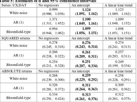
Table 5 reports the estimates of d based on a parametric approach. The model
considered is the following:
yt = α + β t + xt, (1 - L)d xt = ut, t = 1, 2, ...,
where yt stands for the (logged) stock market prices, assuming that the disturbances ut
are in turn a) white noise, b) autoregressive (AR(1), and c) of the Bloomfield-type, the
latter being a nonparametric approach that produces autocorrelations decaying
exponentially as in the AR case.
[Insert Table 5 about here]
We consider the three standard cases of i) no regressors (α = β = 0 above), ii)
with an intercept (i.e., β = 0), and iii) with an intercept and a linear time trend. The most
relevant case is the one with an intercept. The reason is that the t-values imply that the
coefficients on the linear time trends are not statistically significant in all cases, unlike
those on the intercept. We have used a Whittle estimator of d (Dahlhaus, 1989) along
with the parametric testing procedure of Robinson (1994).
The results indicate that for the log UX series the estimated value of d is
significantly higher than 1 independently of the way of modelling the I(0) disturbances.
As for the absolute and squared returns, the estimates are all significantly positive,
[Insert Figure 13 about here]
Figure 13 focuses on the semiparametric approach of Robinson (1995b),
extended later by many authors, including Abadir et al. (2007). Given the nonstationary
nature of the UX series, first-differenced data are used for the estimation, then adding 1
to the estimated values to obtain the orders of integration of the series. When using the
Abadir et al.’s (2007) approach, which is an extension of Robinson’s (1995) that does
not impose stationarity, the estimates were almost identical to those reported in the
paper, and similar results were obtained with log-periodogram type estimators. Along
with the estimates we also present the 95% confidence bands corresponding to the I(1)
hypothesis for the UX data and the I(0) hypothesis for the absolute/squared returns. We
display the estimates for the whole range of values of the bandwidth parameter m = 1, .,,
T/2. It can be seen that the values are above the I(1) interval in the majority of cases,
which is consistent with the parametric results reported in Table 5. For the absolute and
squared returns, the estimates are practically all significantly above the I(0) interval,
implying long memory behaviour. Overall, these results confirm the parametric ones.
The estimated value of d is slightly above 1 for the log stock market prices, and
significantly above 0 for both squared and absolute returns.
[Insert Figure 14 about here]
Figure 14 presents the stability results. We computed the estimates of d with two
different approaches: a recursive one, initially using a sample of 300 observations, and
then adding ten more observations each time, and a rolling one with a moving window
of 300 observations. Persistence appears to decrease over time, especially for the
volatility series.
4. CONCLUSIONS
market indices, namely the PFTS and UX indices. The evidence suggests that this
market is inefficient and that persistence was not constant over time; in particular, it
increased during the recent financial crisis, when the market became less efficient/more
predictable and more vulnerable to market anomalies. This created the opportunity for
profitable trading strategies exploiting the January, day of the week, end of the month,
holidays effects and other market anomalies, or, alternatively, based on following trends
(these issues will be examined in future papers). Finally, our study also shows that data
References
Abadir, K.M., W. Distaso and L. Giraitis, 2007, Nonstationarity-extended local Whittle estimation, Journal of Econometrics 141, 1353-1384.
Dahlhaus, R., 1989, Efficient parameter estimation for self-similar process. Annals of Statistics 17, 1749-1766.
Fox, R. and Taqqu, M., 1986, Large sample properties of parameter estimates for strongly dependent stationary Gaussian time series. Annals of Statistics 14, 517-532.
Geweke, J. and S. Porter-Hudak, 1983, The estimation and application of long memory time series models, Journal of Time Series Analysis 4, 2221-238.
Hurst H. E., 1951. Long-term Storage of Reservoirs. Transactions of the American Society of Civil Engineers, 799 p.
Hurvich, C.M. and B.K. Ray, 1995, Estimation of the memory parameter for
nonstationary or noninvertible fractionally integrated processes. Journal of Time Series Analysis 16, 17-41.
Künsch, H., 1986, Discrimination between monotonic trends and long-range dependence, Journal of Applied Probability 23, 1025-1030.
Lobato, I.N. and C. Velasco, 2007, Efficient Wald tests for fractional unit root. Econometrica 75, 2, 575-589.
Mandelbrot B., 1972. Statistical Methodology For Nonperiodic Cycles: From The Covariance To Rs Analysis, Annals of Economic and Social Measurement 1, 259-290
Peters E. E., 1991, Chaos and Order in the Capital Markets: A New View of Cycles, Prices, and Market Volatility, NY. : John Wiley and Sons, Inc, 228 p
Peters E. E., 1994, Fractal Market Analysis: Applying Chaos Theory to Investment and Economics, NY. : John Wiley & Sons, 336 p
Phillips, P.C. and Shimotsu, K., 2004. Local Whittle estimation in nonstationary and unit root cases. Annals of Statistics 32, 656-692.
Robinson, P. M., 1994, Efficient tests of nonstationary hypotheses. Journal of the American Statistical Association, 89, 1420-1437.
Robinson, P.M., 1995a, Log-periodogram regression of time series with long range dependence. Annals of Statistics 23, 1048-1072.
Robinson, P.M., 1995b, Gaussian semi-parametric estimation of long range dependence, Annals of Statistics 23, 1630-1661.
Sowell, F., 1992, Maximum likelihood estimation of stationary univariate fractionally integrated time series models. Journal of Econometrics 53, 165-188.
Velasco, C. and P.M. Robinson, 2000, Whittle pseudo maximum likelihood estimation for nonstationary time series. Journal of the American Statistical Association 95, 1229-1243.
Velasco, C., 1999a, Nonstationary log-periodogram regression. Journal of Econometrics 91, 299-323.
Velasco, C., 1999b. Gaussian semiparametric estimation of nonstationary time series.Journal of Time Series Analysis 20, 87-127.
Tables and Figures
Table 1: Hurst exponent interval characteristics
Interval Hypothesis Distribution «Memory» of
series Type of process Trading Strategies 0 ≤ H < 0 ,5
Data is fractal,
fractal market
hypothesis is
confirmed
"Heavy tails" of distribution
Antipersistent series,
negative correlation in instruments value changes
Pink noise with
frequent changes in direction of price movement
Trading in the market is more
risky for an
individual participant
H
= 0,5
Data is random, Efficient market
hypothesis is
confirmed
Movement of
asset prices is an example of the random
Brownian motion (Wiener process), time series are normally
distributed
Lack of correlation in
changes in
value of assets
(memory of
series)
White noise of
independen
t random
process
Traders cannot
"beat" the market with the use of
any trading
strategy
0,5 < H
≤
1
Data is fractal,
fractal market
hypothesis is
confirmed
"Heavy tails" of distribution Persistent series, positive correlation within
changes in
the value of assets
Table 2: Hurst exponent estimation for different variants of data filtration
Unfiltered
SMA (2)
SMA (5)
WMA (2)
WMA
(5) Irwin
UX (daily returns) 0.67 0.69 0.73 0.69 0.73 0.70
UX (mixed data) 0.54 0.53 0.54 0.52 0.53 0.49
Random data 0.51 0.56 0.63 0.55 0.61 0.52
[image:17.595.89.516.256.306.2]Mixed random data 0.53 0.52 0.51 0.51 0.51 0.54
Table 3: Hurst exponent estimates with standard methodology (aliquot number of groups) and modified (aliquant number of groups) for different data sets
UX (close) Random UX (SMA 5) UX (WMA 5) UX (Irving)
Standard 0.67 0.51 0.73 0.73 0.7
Modified 0.7 0.55 0.78 0.77 0.73
Table 4: Full-sample analysis of Ukrainian stock market persistence
PFTS UX
Hurst exponent 0,665 0,667
Table 5: Estimates of d and 95% confidence intervals
Series: UX.DAT No regressors An intercept A linear time trend
White noise (0.966, 1.036) 0.999 (1.091, 1.162) 1.124 (1.089, 1.162) 1.123
AR (1) (1.311, 1.452) 1.371 (1.049, 1.161) 1.100 (1.048, 1.152) 1.099
Bloomfield-type (0.944, 1.062) 0.994 (1.056, 1.151) 1.099 (1.051, 1.151) 1.098
SQUARED returns No regressors An intercept A linear time trend
White noise (0.245, 0.316) 0.278 (0.243, 0.314) 0.276 (0.241, 0.313) 0.274
AR (1) (0.218, 0.322) 0.266 (0.209, 0.311) 0.261 (0.203, 0.311) 0.257
Bloomfield-type (0.211, 0.328) 0.254 (0.207, 0.334) 0.251 (0.199, 0.334) 0.249
ABSOLUTE returns No regressors An intercept A linear time trend
White noise (0.239, 0.300) 0.268 (0.229, 0.292) 0.259 (0.228, 0.291) 0.258
AR (1) (0.281, 0.372) 0.326 (0.264, 0.363) 0.311 (0.261, 0.362) 0.309
Figure 1 – Periodisation of financial crisis 2007-2009
18 F igu re 3 Visua l i nter pre
tation of f
[image:20.595.83.296.125.466.2]19 F igu re 4 Vi sua l i nter pre
tation of f
[image:21.595.85.276.86.549.2]20 F igu re 5 Visua l i nter pre
tation of f
[image:22.595.224.450.79.544.2]Figure 6
Visual interpretation of filtered and unfiltered randomly generated data: SMA filtration
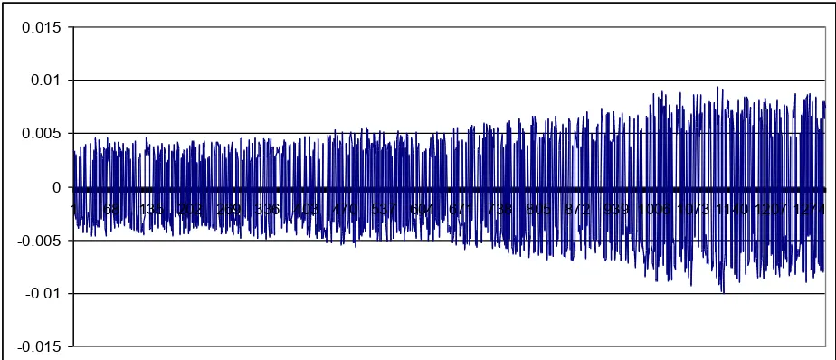
a) Randomly generated data
-0.015 -0.01 -0.005 0 0.005 0.01 0.015
1 68 135 202 269 336 403 470 537 604 671 738 805 872 939 1006 1073 1140 1207 1274
b) Randomly generated data filtered with SMA 2
-0.01 -0.008 -0.006 -0.004 -0.002 0 0.002 0.004 0.006 0.008 0.01
1 68 135 202 269 336 403 470 537 604 671 738 805 872 939 1006 1073 1140 1207 1274
c) Randomly generated data filtered with SMA 5
-0.008 -0.006 -0.004 -0.002 0 0.002 0.004 0.006 0.008 0.01
Figure 7
Visual interpretation of filtered and unfiltered randomly generated data: WMA filtration
a) Randomly generated data
-0.015 -0.01 -0.005 0 0.005 0.01 0.015
1 68 135 202 269 336 403 470 537 604 671 738 805 872 939 1006 1073 1140 1207 1274
b) Randomly generated data filtered with WMA 2
-0.01 -0.008 -0.006 -0.004 -0.002 0 0.002 0.004 0.006 0.008 0.01
1 68 135 202 269 336 403 470 537 604 671 738 805 872 939 1006 1073 1140 1207 1274
c) Randomly generated data filtered with WMA 5
-0.01 -0.008 -0.006 -0.004 -0.002 0 0.002 0.004 0.006 0.008 0.01
Figure 8
Visual interpretation of filtered and unfiltered randomly generated data: Irwin filtration
a) Randomly generated data
-0.015 -0.01 -0.005 0 0.005 0.01 0.015
1 68 135 202 269 336 403 470 537 604 671 738 805 872 939 1006 1073 1140 1207 1274
b) Randomly generated data filtered with Irwin
-0.015 -0.01 -0.005 0 0.005 0.01 0.015
Figure 9: Dynamics of Hurst exponent during 2003-2013
(calculated on PFTS data with “data window” = 300, shift = 10)
Figure 10: Time series UX data
ai) Stock market prices
0 500 1000 1500 2000 2500 3000 3500
08/01/2008 24/05/2013
b) Stock market returns
-0,15 -0,1 -0,05 0 0,05 0,1 0,15 0,2
08/01/2008 24/05/2013
c) Squared market returns
0 0,005 0,01 0,015 0,02 0,025 0,03
08/01/2008 24/05/2013
d) Absolute market returns
0 0,04 0,08 0,12 0,16 0,2
Figure 11: Correlograms
a) Stock market prices
-0,4 -0,2 0 0,2 0,4 0,6 0,8 1 1,2
1 26 51 76 101 126 151 176 201 226 251 276
b) Stock market returns
-0,1 -0,05 0 0,05 0,1 0,15 0,2
1 26 51 76 101 126 151 176 201 226 251 276
c) Squared market returns
-0,1 0 0,1 0,2 0,3 0,4
1 26 51 76 101 126 151 176 201 226 251 276
d) Absolute market returns
-0,2 -0,1 0 0,1 0,2 0,3 0,4
Figure 12: Periodograms
a) Stock market prices
0 3000000 6000000 9000000 12000000 15000000 18000000
1 12 23 34 45 56 67 78 89 100
b) Stock market returns
0 0,0004 0,0008 0,0012 0,0016
1 12 23 34 45 56 67 78 89 100
c) Squared market returns
0 0,000002 0,000004 0,000006 0,000008
1 12 23 34 45 56 67 78 89 100
d) Absolute market returns
0 0,0002 0,0004 0,0006 0,0008 0,001 0,0012
Figure 13: Semiparametric Whittle estimates of d
a) Stock market prices
0 0,4 0,8 1,2 1,6 2
1 102 203 304 405 506 607
b) Squared market returns
-1,2 -0,8 -0,4 0 0,4 0,8 1,2
1 101 201 301 401 501 601
c) Absolute market returns
-1,2 -0,8 -0,4 0 0,4 0,8 1,2
1 101 201 301 401 501 601
The horizontal axis concerns the bandwidth parameter while the vertical one refers to the estimated value of d.
Figure 14: Stability results based on recursive estimates
a) Stock market prices
Adding 10 observation each time Moving windows of 300 observations
1 1,05 1,1 1,15 1,2 1,25 1,3
1 8 15 22 29 36 43 50 57 64 71 78 85 92 99
0,9 1 1,1 1,2 1,3
1 8 15 22 29 36 43 50 57 64 71 78 85 92 99
b) Squared market returns
Adding 10 observation each time Moving windows of 300 observations
0,1 0,15 0,2 0,25 0,3 0,35 0,4
1 8 15 22 29 36 43 50 57 64 71 78 85 92 99
0 0,1 0,2 0,3 0,4 0,5
1 8 15 22 29 36 43 50 57 64 71 78 85 92 99
c) Absolute market returns
Adding 10 observation each time Moving windows of 300 observations
0,1 0,15 0,2 0,25 0,3 0,35 0,4
1 8 15 22 29 36 43 50 57 64 71 78 85 92 99
0,1 0,2 0,3 0,4 0,5