The macroeconomics of immigration

(1)

Munich Personal RePEc Archive

The macroeconomics of immigration

Kiguchi, Takehiro and Mountford, Andrew

Royal Holloway, University of London, Royal Holloway, University of

London

(2)

The Macroeconomics of Immigration

∗ †

Takehiro Kiguchi and Andrew Mountford

Royal Holloway, University of London

March 2013

Abstract

Immigration has been a significant part of US population growth over recent decades, with the number of “foreign born to non-US nationals” rising from approximately 10 million in 1970 to nearly 40 million or 12.9% of the US total population in 2010. In this paper, using a VAR with sign restriction identification, we find that unexpected increases in the working population lead to temporary reductions in GDP per capita and consumption per capita as would be predicted by the standard neoclassical growth model. However they do not lead to increases in non-residential investment or short run decreases in real wages as would also be predicted. The paper shows how a neoclassical growth model with a CES production function where migrant labor and capital are complements to skilled domestic labor and substitutes to each other can produce responses closer to those in the VAR. The paper thus provide support for the microeconometric studies on the impacts of immigration which found that immigrant labor is complementary to, rather than a substitute for, most native labor.

Keywords: Macroeconomics, Immigration

JEL Classification Numbers: O40, F11, F43.

∗_{We thank}

†_{Address for correspondence: Andrew Mountford, Dept. Economics, Royal Holloway College, University of London,}

(3)

1 Introduction

While there have been a lot of recent studies on the microeconomic impacts of immigra-tion there has been less attenimmigra-tion focussed on the implicaimmigra-tions of immigraimmigra-tion for the macroeconomy. According to US Census Bureau and Current Population Survey (CPS) data, immigration has been a significant part of the US population growth over recent decades. In 1970 about 9.6 million (4.7%) of the US total population was foreign born to non-US nationals, by 2010 this number had risen to nearly 40 million or 12.9% of the US total population. In this paper we examine the effect of shocks to working population on the macroeconomy using the techniques of macroeconomic time series analysis. The analysis shows that, consistent with the standard neoclassical growth model, GDP per capita and consumption per capita temporarily fall in response to a positive shock to the working population. However non-residential investment per capita does not rise and real wages do not fall in the short run following an unexpected increase in the working population and as would also be predicted by the standard growth model.

The paper shows that a neoclassical growth model with a CES production func-tion where migrant labor is a substitute for capital but a complement to skilled domestic labor can produces responses to an immigration shock much closer to those of the VAR. In particular it can produce responses where investment falls in response to an immigra-tion shock and where the wage response of most agents is initially positive due to the complementarity of immigrant labor with most domestic labor. Thus the VAR results and the macroeconomic growth model both lend support to the findings of the microe-conomic literature that immigrant labor is a much closer substitute for native unskilled labor than native skilled labor, see for example Ottaviano and Peri (2012) for the US Economy and Manacorda, Manning and Wadsworth (2012) for the UK economy.

(4)

levels. We therefore interpret shocks to unanticipated changes in the working population as immigration shocks.

The analysis and results of the paper are of interest for two distinct reasons. Firstly the key state variable in balanced growth models is the capital labor ratio and while the literature has paid a lot of attention to the determinants of individual labor supply1

much less attention has been given to the determinants of the size of the working pop-ulation, although see Doepke, Hazan and Maoz (2012) for a notable exception. This paper attempts to redress this imbalance by focussing on the macroeconomic effects of immigration which is one of the key determinants of changes in the labor force. Secondly there is a large microeconomic literature on the effects of immigration on the Labor mar-ket. One of the key puzzles of this literature was the finding that immigration has only a small effect on aggregate wages, with only the wages of the least skilled workers being adversely affected by immigration.2 _{This paper, using a very different methodology and}

different, macroeconomic, data provides macroeconomic support for this analysis by also finding that immigration shock is not empirically associated with short run decreases in aggregate wage rates.

The paper is organized as follows. In section 2 we present and discuss the raw data. In Section 3 we present results from the VAR analysis and in Section 4 we discuss to what extent the standard macroeconomic growth model can be adapted to explain these results.

2 Trends in Population Growth and Immigration

This section presents the data we will be using below in our VAR analysis. One con-tribution of this section is to compute an unanticipated change in population variable by removing anticipated changes in the working population caused by publicly recorded changes in the birth and mortality rates. This is important and interesting for two rea-sons. Firstly because controlling for predictable changes in variables in a VARs is nec-essary to remove bias, as the work of Ramey (2011) and Auerbach and Gorodnichenko (2012) detail. Secondly when we do construct this series it corresponds quite closely to immigration level which is intuitive. Thus in the VAR section below we interpret the

1

For surveys of the literature see e.g. Uhlig (1999) or Christiano, Eichenbaum and Evans (2005)

2

(5)

0

1

2

3

4

Millions

1950 1970 1990 2005

Date Change in Working Population

0

1

2

3

4

5

Millions

1950 1970 1990 2005

[image:5.595.81.570.78.338.2]

Date Number of Live Births 16 Years Previously

Figure 1: Live Births 16 years previously are a major and predictable influence on the Working Population

shocks to unanticipated population as immigration shocks.

Figure 1 plots the changes in the rate of growth of the working population and the number of live births 16 years previously. It shows that they are highly related, although not perfectly correlated. VAR analysis assumes that the errors in the VAR are orthogonal to information contained in the past values of the variables in the VAR, see for example Canova (2007). Thus it is necessary to remove this predictable element from the population series, see for example the discussion in Ramey (2011) and Auerbach and Gorodnichenko (2012). We do this by constructing an unanticipated change in population series, W P opU

t , to correct for these predictable effects, using the following

formula

W P opU

t = W P opt−W P opAt

where W P opAt = (1−δt65−₁ −mort

16−₆₄

t−₁ )W P opt−₁+ (1−mort1 −₁₅

t−₁₆)Birthst−₁₆

where the W P opt is the series for working population in the US is taken from

Coci-uba, Prescott and Ueberfeldt (2009). W P opA

(6)

−.5

0

.5

1

1.5

2

Percent

1950 1970 1990 2005

Date Unanticipated Changes in Working Population

−.5

0

.5

1

1.5

Percent

1950 1970 1990 2005

[image:6.595.85.536.78.333.2]

Date New Permanent Residents

Figure 2: Unanticipated changes in Population and Census Department Figures on New Permanent Residents

time which is equal to the previous year’s working population minus an estimate of the proportion aged 64 who will retire, δ65

t−1, and an estimate of the mortality rate of the

working population plus the births from 16 years previously also adjusted for mortality. The data used is all freely and publicly available on the internet. That for mortality rates and birth rates are taken from 5 yearly samples from the CDC/NCHS National Vital Statistics and data on the age distribution is taken from decennial census data. Linear interpolation is used to generate annual numbers for mortality rates.

(7)

workers to apply for permanent resident status after a period of three years.3 _{The passing}

of the act also coincided with a period of high Mexican unemployment and so caused many temporary workers who would otherwise have returned to their country of origin to remain in the United States and become permanent residents. It is estimated that 2.3 million Mexicans took advantage of this possibility, see Durand, Massey and Parrado (1999). The gradual track to permanent residency also explains why the peak of the new permanent residents series occurs after that for the changes in working population series.

The series are also similar in scale. Over the sample period 1950-2005 the cu-mulative unanticipated changes in the working population is approximately 38.2 million with 17.8 million occurring since 1990. The corresponding numbers for the new perma-nent residents series are 31.9 million and 15.7 million. One should not expect a perfect correspondence between these two figures since one can attain new permanent resident status and not be part of the working population and vice versa. However the similarity between the two series is reassuring. Figure 2 also plots the NBER business cycle dates with the recessions shaded in gray. It is noticeable that the response of the unanticipated changes in working population is more volatile and reactive to recessions than the series for new permanent residents which is intuitive.

3 VAR Analysis

3.1 Description of the VAR

We use an 8 dimensional VAR with annual data from 1950 to 2005 for the following variables; GDP, private consumption, non-residential investment, residential investment, hours worked, real wages and the two immigration series, the numbers of new permanent residents and the constructed unanticipated population variable described above.4 _All

variables are real and, with the exception of the wage series, expressed as per capita of

3

This is known as the Special Agricultural Workers provision.

4

(8)

[image:8.595.158.459.112.217.2]

TABLE 1

IDENTIFYING SIGN RESTRICTIONS

GDP Non-Res Hours Unantipated Cons Invest Working Pop.

Business Cycle + + +

Population +

This table shows the sign restrictions on the impulse responses for each identified shock. ‘Non-Res Inv’ stands for Non-Residential Investment. A ”+” means that the impulse response of the variable in question is restricted to be positive for two years following the shock, including the year of impact. A blank entry indicates, that no restrictions have been imposed.

the working population. The VAR has 2 lags, no constant or a time trend, and uses the logarithm for all variables except for the population variables where we have used the level.

The VAR in reduced form is given by

Yt =

2

X

i=1

BiYt−i+ut , t= 1,· · · , T, E[utu

′

t] = Σ

whereYtare 8×1 vectors, 2 is the lag length of the VAR,Bi are 8×8 coefficient matrices

and ut is the one step ahead prediction error.

3.2 Identification

The problem of identification is to translate the one step ahead prediction errors, ut,

into economically meaningful, or ‘fundamental’, shocks, vt. In this paper we identify

shocks using the sign restriction approach of Uhlig (2005) and Mountford and Uhlig (2009). Identification in this methodology amounts to identifying a matrixA, such that

ut=Avt and AA′ = Σ. Each column of A represents the immediate impact, or impulse

(9)

horizonk then the criterion function, Ψ(a), is

Ψ(a) = X

jǫJS,+

1

X

k=0

f(−rja(k)

sj

) + X

jǫJS,−

1

X

k=0

f(rja(k)

sj

)

where f is the function f(x) = 100x if x≥ 0 and f(x) =x if x ≤0, sj is the standard

error of variable j, JS,+ is the index set of variables, for which identification of a given

shock restricts the impulse response to be positive and JS,− is the same for variables

restricted by identification to be negative. Since we use annual data we only restrict the signs of the impulses for two periods i.e. for the two years after the shock. When multi-ple shocks are identified there is an additional constraint on the minimization that the identified shock be orthogonal to previously identified shocks, as detailed in Mountford and Uhlig (2009).

In this paper we use two identification schemes. We first only identify the unantic-ipated population/immigration shocks and then we identify two shocks, first a business cycle shock and then the unanticipated population/immigration shock. Table 3.2 pro-vides a description of the identifying sign restrictions for these shocks. The advantage of the penalty function approach is that, by rewarding larger responses of the correct sign, it gives the shock identified first the greatest opportunity to explain the variation in the data. Thus when the unanticipated population/immigration shock is identified second it is restricted to explaining the variation in the data left over after the variation explained by the business cycle shock has been taken out. As well as a robustness exercise this identification scheme is interesting in its own right, as it should also pick up temporary variations in immigration which may be associated with business cycle fluctuations.

3.3 Empirical Results

(10)

−2 −1 0 1 2 Percent

0 4 8 12 16

Date GDP −2 −1 0 1 2 Percent

0 4 8 12 16

Date CONSUMPTION −5 −3 1 0 1 3 5 Percent

0 4 8 12 16

Date RESIDENTIAL INVESTMENT −5 −3 1 0 1 3 5 Percent

0 4 8 12 16

Date NON−RESIDENTIAL INVESTMENT −2 −1 0 1 2 Percent

0 4 8 12 16

Date AVERAGE HOURS −2 −1 0 1 2 Percent

0 4 8 12 16

Date REAL WAGES −2 −1 0 1 2 Percent

0 4 8 12 16

Date NEW PERMANENT RESIDENTS

−2 −1 0 1 2 Percent

0 5 10 15

[image:10.595.191.421.74.421.2]

Date UNANTICIPATED POPULATION

Figure 3: Impulse Responses to an Immigration Shock Ordered First.

3.3.1 The Immigration Shock Ordered First

(11)

−2 −1 0 1 2 Percent

0 4 8 12 16

Date CONSUMPTION −5 −3 1 0 1 3 5 Percent

0 4 8 12 16

−2 −1 0 1 2 Percent

0 4 8 12 16

[image:11.595.192.421.74.421.2]

Figure 4: Impulse Responses to a Business Cycle Shock Ordered First.

that would be predicted by a standard growth model where wages fall on impact after an unexpected increase in its labor force. Finally note that the response of the new permanent residents to the immigration shock is intuitive. It is much smoother than the responses of the unanticipated population variable which is intuitive and consistent with the view that the unanticipated working population variable will contain more temporary immigrants than the new permanent residents series.

3.3.2 The Immigration Shock Ordered Second

(12)

−2 −1 0 1 2 Percent

0 4 8 12 16

Date CONSUMPTION −5 −3 0 3 5 Percent

0 4 8 12 16

−2 −1 0 1 2 Percent

0 4 8 12 16

[image:12.595.191.422.74.422.2]

Figure 5: Impulse Responses to an Immigration Shock Ordered Second After a Business Cycle Shock

the variation attributed to one identified shock may actually be due to another shock. In macroeconomics the business cycle shock is commonly felt to be an important source of variation and so as a robustness check it is interesting to see whether the responses to the immigration shock change significantly once the business cycle variation is accounted for

5_{. Secondly, it is often thought immigration reacts to the business cycle and that while}

the stage of the business cycle should not matter for permanent immigrants temporary migrants may be affected by the state of the business cycle.

Figure 4 displays the responses to the Business Cycle shock. These responses of the non-population variables are as expected and very similar to those in Mountford and Uhlig (2009) The responses of all the macro variables are positive and persistent. The

5

(13)

population variables both show cyclical variation in response to the business cycle shock although with a lag. The immigration response is negative on impact before rising and becoming significantly positive after three years after the shock. The new permanent residents series shows the same pattern but is a much smaller response and so insignificant for all horizons after impact.

Figure 5 shows the impulse responses of the Immigration shock identified after the business cycle shock. What is striking is how similar the responses are to those in Figure 3. This means that the restriction to be orthogonal to the business cycle shock hardly binds at all which is consistent with the most of the variation in immigration not being influenced by the business cycle. The main differences between Figures 5 and 3 are that the error bands around consumption are tighter and the responses of real wages appears less negative in Figures 5 .

3.3.3 Adding Labour Share

In Figures 6 and 7 we substitute a Labor share variable in to the VAR in place of the real wage rate. The variable is the Nonfarm Business Sector: Labor Share, series PRS85006173, from the Bureau of Labor Statistics. This is interesting as a robustness check and also because an increase in the ability of immigrant labor may reduce the bargaining power of labor and so reduce labor share, see Kiguchi (2013). These Figures do indeed show evidence that over the medium term labor share does decline in response to an immigration shock. Thus the medium term responses of wages and labor share do seem to differ from their short term effects. This is a large issue see for example the work of Duenhaupt (2011), Heathcote, Perri and Violante (2010) and Piketty and Saez (2003, 2006) and which is beyond the scope of this paper, but it is certainly an exciting area for further research.

4 A Growth Model with Immigration Shocks

(14)

−2 −1 0 1 2 Percent

0 4 8 12 16

Date LABOR SHARE −2 −1 0 1 2 Percent

0 4 8 12 16

−2 −1 0 1 2 Percent

0 5 10 15

[image:14.595.192.421.74.422.2]

Figure 6: Impulse Responses to an Immigration Shock Ordered First With Labor Share.

(15)

−2 −1 0 1 2 Percent

0 4 8 12 16

Date LABOR SHARE −2 −1 0 1 2 Percent

0 4 8 12 16

−2 −1 0 1 2 Percent

0 4 8 12 16

[image:15.595.191.422.75.420.2]

Figure 7: Impulse Responses to an Immigration Shock Ordered Second after a Business Cycle Shock with Labor Share.

sharing within the household , see e.g. Gal´ı (2011) or Br¨uckner and Pappa (2012). Intuitively one can think of the household as a composite representative agent made up of a certain proportion of skilled and unskilled labor which can only be supplied together. This is a simplifying assumptions that allows the model to be solved in a standard way. There are clearly possible extensions of the model, such as allowing Household members to differ in some dimension, as in Gal´ı (2011) and Br¨uckner and Pappa (2012), but this is not necessary for the purpose of this paper.

(16)

the following form

U =E

" ∞

X

t=0

βt_N tut

#

where Nt is the number of agents in each household, β, the discount factor, and where

ut is given by

ut=

(ctΦ(lt))1−η −1

1−η

with ct denoting per capita consumption, lt denoting per capita labor supplied, 1/η

>0 the intertemporal elasticity of substitution, and Φ(lt) a strictly positive, decreasing,

concave and thrice differentiable function. We will assume that Φ(lt) is such that there is

a constant Frisch Elasticity of labor supply with respect to the wage rate, see Trabandt and Uhlig (2011). As mentioned above we will assume that the representative household is a composite of both types of labor, skilled and unskilled, which it can only supply together so thatls,t =lu,t=ltwherels,tandlu,tis the labor supply of skilled and unskilled

household member’s respectively. The proportion of skilled labor in the representative household’s composite labor is the same proportion as in the economy, λs

t, where λst =

Ns,t/Nt and Nt = Ns,t +Nu,t. The representative agent’s labor supply decision is to

chooselt subject to the weighted average wage, wt= (ws,tλst+wu,tλut). The Household’s

budget constraint is in each period therefore

ctNt+xtNt=wtltNt+rtktNt

where xt is investment per person, kt is the capital per person, wt is the wage rate and

rt is the capital rental rate. Capital accumulates via investment thus

kt+1Nt+1 = (1−δ)ktNt+xtNt

Production takes place under perfect competition and constant returns to scale according to a CES production function. We use the standardized function form as in Cantore, Ferroni, and Le´on-Ledesma (2011),

yt=

"

α

kt

k

σ−1

σ

+ (1−α)

Atltλut

λu_l

σ−1

σ

# θσ

σ−1

Atltλst

λs_l

1−θ

whereyt=Yt/Nt, and we assume that the level of technology, At, augments both skilled

(17)

between capital and unskilled labor, and the capital intensity in production respectively. Factor prices are determined by factors marginal products so that

rt =

yt

kt

θα(kt

k)

σ−1

σ

[α(kt

k)

σ−1

σ + (1−α)(Atltλ u t

λu_l ) σ−1

σ ]

wu,t = θ

yt

ltλut

(1−α)(Atltλut

λu_l ) σ−1

σ

[α(kt

k)

σ−1

σ + (1−α)(Atltλ u t

λu_l ) σ−1

σ ]

ws,t = (1−θ)

yt

ltλst

The stochastic processes driving technological progress and population growth are

At

At−₁

= ζtA,

Nt

Nt−₁

= ζN t

where ζA

t and ζtN are both stationary stochastic processes with mean ζA and ζN

re-spectively.

Finally the market clearing/feasibility constraint is given by

ct+xt=yt.

4.1 Modeling Immigration Shocks

We model an immigration shock as a shock which leads to an increase in the proportion of unskilled labor in the economy, λu

t, as well an increase in the working population.

We use a broad definition of skills and set λs _{= 0}_._{9 which is justified by the fact that}

90% of young people graduate from high school in the US, although clearly alternative interpretations and calibrations are possible. Given this if at the steady state the working population increases by a% and all of this increase is in unskilled workers then the new share of unskilled workers will rise to λu,newt = (100λu + a)/(100 + a) and so cλut =

(100a(1−λu₎₎_/_{(100 +}_a₎_λu6_{. Thus an immigration shock in our model is a simultaneous}

shock to both population , ζN

t , and also to λut . The proportion of unskilled amongst

immigrants can be varied so that the size of the response of cλu

t also varies. This is

discussed below. 6

(18)

0 1 2 3 4 5 6 7 8 9 −1

−0.5 0 0.5 1

Output

0 1 2 3 4 5 6 7 8 9 −1

−0.5 0 0.5 1

Consumption

0 1 2 3 4 5 6 7 8 9 −2

−1 0 1 2

Capital

0 1 2 3 4 5 6 7 8 9 −1

−0.5 0 0.5 1

Investment

0 1 2 3 4 5 6 7 8 9 −0.5

0 0.5

Hours

0 1 2 3 4 5 6 7 8 9 −2

−1 0 1 2

Aggregate Wage

0 1 2 3 4 5 6 7 8 9 −10

−5 0

years Wages for Skilled and Unskilled Labor

Skilled Unskilled

0 1 2 3 4 5 6 7 8 9 −1

−0.5 0 0.5 1

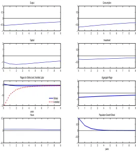
[image:18.595.173.445.95.398.2]

years Population Growth Shock

Figure 8: Impulse Responses to an Immigration Shock – a shock where population rises and the proportion of unskilled workers in the labor force also rises.

4.2 Log-Linearizing around the Balanced Growth Path

In order to be able to log-linearize around the steady state, we need to detrend variables on the balanced growth path. Following Uhlig (2010) we will denote log-deviations by hats so that _bct = log(cet)−log(c) = (cet− c)/c where cet ≡ ct/At and c is the steady

state of c_et. Thus noting that λbtu =−(λs/ λu)λbst and that wt= (ws,tλst +wu,tλut) and so

b

wt = ηs(wbs,t+λbst) + (1−ηs)(wbu,t−λbst) where ηs = wsλs/w and w =wsλs+wuλu, we

(19)

[image:19.595.81.585.122.267.2]

TABLE 2

LOG-LINEARIZED EQUATIONS OF THE MODEL

b

yt = θ[αbkt+ (1−α)(lbt+bλut)] + (1−θ)(blt+bλst) byt = (c/y)bct+ (x/y)xbt

b

wu,t = byt−(blt+λbut)−α σ

−₁

σ bkt+α( σ−₁

σ )(blt+bλut) wbs,t = byt−(blt+λbst)

b

rt = byt−bkt+ (1−α)(σ

−₁

σ )bkt−(1−α)( σ−₁

σ )(blt+bλ u

t) wbt = _ω1_Sblt+bct

b

kt+1 = (1

−δ)

ζN_ζAbkt+

h

1−(1−δ)

ζN_ζA

i b

xt−ζbtA+1−ζbtN+1 λbt = −ηbct−(1−η)κblt

b

wt = ηs(wbs,t+bλst) + (1−ηs)(wbu,t+bλtu) 0 = Et[bλt+1−λbt−ηζbtA+Rbt+1]

b

Rt = (1−β(1−δ)(ζA)−η)rbt bλut = −(λs/λu)bλst

b

ζA

t = ρAζbtA−₁+εA,t ζb

N

t = ρNζbtN−₁+εN,t

This table shows the equations of the log-linearized version of the model

4.2.1 Choosing Parameters

On the balanced growth path lt+1 = lt = l and ct+1 = ζAct. Hence the first order

conditions imply that 1 =Et[(ζA)−ηβ(1 +r−δ)]

r = (ζ

A₎η

β −(1−δ).

Following Uhlig (2010) and Trabandt and Uhlig (2011) we set the expected annual rate of growth of technology to be ζA _{= 1}_._{02, the depreciation rate to be} _δ _{= 0}_._{07, and}

the interemporal elasticity of substitution is set at 0.5 hence η = 2. The discount rate

β = 0.998 hence R ≡ (1 +r −δ) = (ζA₎η_/β _{= 1}_.₀₄₀₄_/₀_._{998 = 1}_._{042. From above}

we know that r = θαy/k and so given calibrated value for θ, and α and given that

r= (ζA_β)η−(1−δ) we will have an expression fory/k . Thus ifθ = 0.4 and α= 0.9 then

y/k = 0.112/0.36 = 0.312 hence k/y = 3.20. The capital accumulation equation in the steady state givesx/y = (k/y)[ζN_ζA₋₍₁₋_δ_{)] = 3}_._20[1_.₀₁₂_×₁_.₀₂₋₀_._{93] = 0}_._{327 which}

is similar to that in Trabandt and Uhlig (2011) and which implies that c/y= 0.673.

4.3 Impulse Responses

(20)

0 1 2 3 4 5 6 7 8 9 −1

−0.5 0 0.5 1

Output

0 1 2 3 4 5 6 7 8 9 −1

−0.5 0 0.5 1

Consumption

0 1 2 3 4 5 6 7 8 9 −2

−1 0 1 2

Capital

0 1 2 3 4 5 6 7 8 9 −1

−0.5 0 0.5 1

Investment

0 1 2 3 4 5 6 7 8 9 −0.5

0 0.5

Hours

0 1 2 3 4 5 6 7 8 9 −2

−1 0 1 2

Aggregate Wage

0 1 2 3 4 5 6 7 8 9 −1

−0.5 0 0.5

years Wages for Skilled and Unskilled Labor

Skilled Unskilled

0 1 2 3 4 5 6 7 8 9 −1

−0.5 0 0.5 1

[image:20.595.173.445.94.399.2]

years Population Growth Shock

Figure 9: Impulse Responses to a pure Population Shock – a shock where population rises and the proportion of skiiled and unskilled workers is unchanged.

section 4.1. In Figure 9 by way of contrast we present the impulse of a pure population shock which is a positive shock to the rate of population growth with no change in the proportion of unskilled workers in the economy.

(21)

shock, 8 investment falls as the increased in unskilled labor substitutes for capital in the production function. The response of unskilled wage rates also differs greatly between the two cases with unskilled wages falling sharply in response to an immigration shock while skilled wages initially rise in response to the immigration shock before falling slightly.

The responses to the immigration shock in Figure 8 are much closer to the VAR responses of Figure 3 and Figure 5 than those of 9. However they are clearly not a perfect fit. The most notable discrepancy is that aggregate wages still fall in response to an immigration shock. It is interesting to note however that the skilled wage does initially rise in response to an immigration shock before falling which is indeed the qualitative response of the wage variable in the VAR. Note that in our calibration 90% of labor is skilled labor and so if the wage variable in the VAR - Nonfarm Business Sector wage rate - has a greater skill component than the economy as a whole, or if immigrants wages do not make it onto the official wage data then the equivalent variable to the VAR in this model would indeed be the skilled wage responses. However we do not model an informal sector in this paper and so again we leave this as a potential fruitful avenue for further research.

Conclusion

(22)

References

[1] Auerbach, A., and Y. Gorodnichenko (2012). “Fiscal Multipliers in Recession and Expansion,” NBER Chapters, in: Fiscal Policy after the Financial Crisis National Bureau of Economic Research, Inc.

[2] Br¨uckner, M., and E. Pappa (2012). “Fiscal Expansions, Unemployment and Labor Force Participation,” International Economic Review, Vol 53(4), 1205-1228.

[3] Cahuc, P., and A. Zylberberg, (2004). Labor Economics, MIT Press.

[4] Cantore, C., F. Ferroni, and M.A. León-Ledesma (2012). “The dynamics of hours worked and technology,” Banco de España Working Papers 1238, Banco de España.

[5] Canova, F. (2007). Methods for Applied Macroeconomic Research, Princeton Uni-versity Press.

[6] Christiano, L., M. Eichenbaum, and C. Evans (2005), “Nominal rigidities and the dynamic effects of a shock to monetary policy,” Journal of Political Economy, Vol. 113(1), 1-45.

[7] Cociuba, S., E. Prescott, and A. Ueberfeldt (2009). “U.S. Hours and Productivity Behavior Using CPS Hours worked Data: 1947-III to 2009-III,” Mimeo.

[8] Doepke, M., M. Hazan, and Y. Maoz (2012). “The Baby Boom and World War II: A Macroeconomic Analysis. Working paper Northwestern University.

[9] Duenhaupt P. (2011). “The Impact of Financialization on Income Distribution in the USA and Germany: A Proposal for a New Adjusted Wage Share,” IMK working Paper, Hans B¨ockler Foundation.

[10] Durand, J., D. Massey, and E. Parrado (1999). “The New Era of Mexican Migration to the United States. Journal of American History Vol. 86(2), 518-536.

[11] Dustmann, C., T. Frattini, and I. P. Preston (2008). “The Effect of Immigration along the Distribution of Wages,” CReAM Discussion Paper No.03/08.

[12] Gal´ı J. (2011).Unemployment Fluctuations and Stabilization Policies: A New Key-nesian Perspective, Princeton University Press.

[13] Heathcote, J., F. Perri, and G. L. Violante (2010). “Unequal We Stand: An Empir-ical Analysis of Economic Inequality in the United States: 1967-2006”, Review of Economic Dynamics, Vol13(1), 15-51.

[14] Kiguchi, T. (2013). “Bargaining and Immigration in a Macro Model,” Mimeo, Royal Holloway, University of London.

[15] L¨utkepohl, H. (2005).New Introduction to Multiple Time Series Analysis, Springer.

(23)

[17] Mountford, A., and H. Uhlig (2009). “What are the effects of fiscal policy shocks?.”

Journal of Applied Econometrics, Vol. 24(6), 960-992.

[18] Ottaviano G. I. P., and G. Peri (2012). “Rethinking the Effect of Immigration on Wages,” Journal of the European Economic Association, Vol. 10(1), 152-197.

[19] Piketty T., and E. Saez (2003). “Income Inequality in the United States, 1913-1998,”

Quarterly Journal of Economics, Vol. 118(1), 1-39.

[20] Piketty, T., and E. Saez (2006). “The evolution of top incomes: A historical and international perspective,” American Economic Review, Papers and Proceedings, Vol.96(2), 200-205.

[21] Ramey, V. (2011). “ Identifying Government Spending Shocks: It’s all in the Tim-ing,” Quarterly Journal of Economics, Vol. 126(1), 1-50.

[22] Trabandt, M., and H. Uhlig (2011). “The Laffer Curve Revisited,”Journal of Mon-etary Economics, Vol. 58(4), 305327.

[23] Uhlig, H. (1999). “A Toolkit for Analyzing Nonlinear Dynamic Stochastic Models Easily,” In R. Marimon and A. Scott, editors Computational Methods for the Study of Dynamic Economies, 30-61.

[24] Uhlig, H. (2005). “What are the effects of monetary policy on output? Results from an agnostic identification procedure,” Journal of Monetary Economics, Vol. 52(2), 381-419.

[25] Uhlig, H. (2010). “Some Fiscal Calculus,” American Economic Review, Papers and Proceedings, American Economic Association, Vol. 100(2), 30-34.