Conjugate Heat Transfer in a Developing Laminar Boundary Layer



Abstract—For steady-state conditions, the conjugate heat transfer process for a developing laminar boundary-layer flow over a heated plate is considered. Boundary conditions for the heated plate are set as Neumann, i.e., constant heat flux for the bottom of the plate, and as convective heat transfer for the top, with the interface temperature obtained using Chebyshev polynomial approximations. Computation of the derived equations is by the computer algebra system, Mathematica.

Index Terms—Conjugate heat transfer, Chebyshev polynomials.

I. INTRODUCTION

LOW and heat transfer in boundary layers, both laminar and turbulent have been investigated for many years both experimentally and numerically [1,2]. Quite often in the design of electronic boxes, the boundary layers over flat components are either laminar or transitional in nature [3-5]. Chebyshev polynomials have been used extensively in the calculation of radiative heat transfer [6,7] and to some extent in convective heat transfer [8], while conjugate heat transfer has been researched within the field of computational fluid dynamics [8-11].

In this work the aim is to simultaneously solve both heat conduction, as found in a solid heated plate and the convective heat transfer as found in the boundary layer above. The link between these two regimes is facilitated using a linear combination of Chebyshev polynomials.

II. HEATANDMASSTRANSFEREQUATIONS

Assumptions for the boundary-layer flow here are that the fluid is steady, incompressible, the properties of the fluid are constant, the flow remains in the laminar regime and that the flow is two-dimensional, i.e., the span of the flat plate is infinite. Also, the assumptions are that the pressure gradient along the -axis, i.e., the free-stream direction is negligible, and, that no body forces act on the fluid. The Navier-Stokes equations for the boundary-layer reduce to,

Manuscript received March 4, 2014; revised March 25, 2014. D. Adair is with the School of Engineering, Nazarbayev University, Astana, 010000, Republic of Kazakhstan (phone: +7 7172 706531, e-mail: dadair@ n.edu.kz).

T. Alimbayev is with the School of Engineering, Nazarbayev University, Astana, 010000, Republic of Kazakhstan (e-mail: [email protected]).

, (1)

and the continuity equation to,

0. (2)

Since there is no pressure gradient within the boundary layer, the energy equation is that of isobaric flow, i.e.,

. (3)

The term / is much smaller in magnitude than / and it is convenient to divide through the equation by , giving the following energy equation for steady, two-dimensional, isobaric flow,

, (4)

where, / . Within the solid plate the Laplace equation applies for the energy equation,

0. (5)

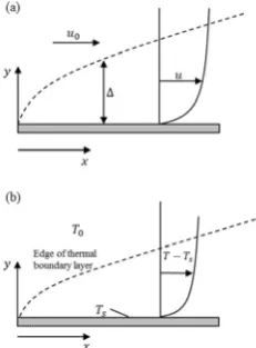
A schematic of both the mass and heat transfer is shown on Fig. 1.

Fig. 1 Schematic of (a) mass and (b) heat transfer in a laminar boundary-layer over a flat heated plate.

Conjugate Heat Transfer in a Developing

Laminar Boundary Layer

Desmond Adair and Talgat Alimbayev

Equations (1,2,4,5) are now non-dimensionalised using,

, , , ,

, , ,

where, is the heat flux through the bottom of the plate. This leads to,

′ ′

′ ′

′ ′

1 ′

′ , (6)

′ ′

1 ′

′

′ 0, (7)

′ ′ ′ ′

1

′ , (8)

1

′ ′ 0. (9)

Here, and are the Reynolds and Peclet number respectively, based on the streamwise length of the plate. The equivalent non-dimensionalised boundary conditions are,

0 ′ 1 and 1: 0; 0 ′ 1

→ ∞: 1, 0

0 ′ and → ∞: 0

0 1 and 1: , ⁄ ′ ′ ⁄ ′

0 1 and 0: ⁄ 1

0 and 1: 1, 0

0 and 1: 0

0 and 0 1: ⁄ 0

1 and 0 1: ⁄ 0 (10)

III. CHEBYSHEVPOLYNOMIALSOFTHEFIRST

KIND

The Chebyshev polynomials can be obtained by means of the Rodrigue’s formula,

2 !

2 ! 1 1

0,1,2,3 … …

(11)

When the first two Chebyshev polynomials and are known, all other polynomials, , 2 can be obtained by means of the recurrence formula,

2 (12)

The Chebyshev polynomials of the first kind are orthogonal in the interval 1,1 and the orthogonally properties for these polynomials can be determined using knowledge of the orthogonal properties of cosine functions,

cos cos d

0

2 0 .

0

(13)

Then on substituting,

cos , cos

to obtain the orthogonal properties of the Chebyshev polynomials,

d √1

0

2 0

0

,

it can be seen that the Chebyshev polynomials form an orthogonal set on the interval 1,1 with the weighting function 1 ⁄ _{. If needed it is possible to map}

1,1 to a general range of interest , using

2 ⁄ where is within the range , .

When Chebyshev polynomials are considered over discrete points, the continuous function is replaced by a set of discrete values of the function at these points. It can be

shown that the Chebyshev polynomials are

orthogonal over the following discrete set of 1 points , equally spaced on ,

0, , , … , 1 , where, cos .

This leads to,

1

2 1 1

1

2 1 1

0

2 0

0

(15)

The are also orthogonal over the following points equally spaced,

, , , … , where cos

0

2 0

0

(16)

The set of points are clearly the midpoints of of the first case. The unequal spacing of the points in

compensates for the weight factor, 1 ⁄ _.

cos 1

2 _{, 1,2, … , . (17)}

A function can be approximated [13] by an n-th

degree polynomial expressed in terms of , … , ,

⋯ 1

2 18

2

, 0,1, … , (19)

and, , 1, … , 1 are zeros of . From the basic

definition, cos cos we have,

cos cos cos

1 2

1 . (20)

In this work, the temperature at the interface is represented as a linear combination of Chebyshev polynomials,

, 1

2 (21)

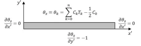
IV. HEATCONDUCTIONINTHESOLIDPLATE Boundary conditions for the heat conduction in the solid plate are summarized on Fig. 2.

Fig. 2 Boundary conditions for the heated solid plate.

The boundary conditions in the y’- direction are in fact

non-homogeneous which necessitates translation of the function as,

, , 1 (22)

The general solution for heat flow within the solid is well known and is,

, ∙ cos cosh (23)

The coefficients can be obtained using the boundary conditions found at the solid/fluid interface by setting (22)

equal to , where ≡ 2 ∙ 1 when 1.

When the orthogonal properties of Chebyshev polynomials in the range 1,1 it can be shown that,

4 1 , (24)

and, when 0,

2 cos d ′

cosh . (25)

Using (21) a solution for the temperature distribution within the solid can be given as,

, =

2 ∑ cosh cos cos d

cosh

1 (26)

V. ANALYSISATTHESOLID/FLUIDINTERFACE The energy balance at the interface can be given as [2],

/ , (27)

where ′′

, . In non-dimensional terms,

, ′ , (28)

The local Nusselt number is,

⇒ ⇒

′ ′ ′ ,

(29)

where is the local Biot number in non-dimensional coordinates. is found by putting the Chebyshev polynomial solution (21) into (28) to obtain (30).

(30)

∑ sinh cos cos d ′

cosh

where, 1 2 . The local Nusselt number can then be found from (29). The average convective heat transfer can be found at the surface using suggestions by [14], i.e.

1

, , d (31)

, 1 d

2 d ̅

(32)

and on using the orthogonal properties of Chebyshev polynomials,

, . (33)

Starting with (30) and (31), (34) can be found,

, d 34

1 2 ′ cos

∙ tanh cos d d ′

and using the properties of the Chebyshev polynomials,

, d (35)

it can be found that,

∑ _{2 1 2 1}

1

∑ _{2 1 2 1} (36)

1

∑ _{2 1 2 1} .

The temperature distribution at the solid/fluid interface is now specified in terms of a polynomial. In this work only the quadratic and cubic were used. So the temperature in non-dimensional terms at the interface can be represented by,

⋯

′ ′ ⋯ ′

≡ ⋯ 1

2

The relationships for quadratic and cubic coefficients are,

TABLEI

CHEBYSHEVPOLYNOMIALSPARAMETERCOEFFICIENTS

C

1/2 3/8 - 1/2 1/2 - - 1/8 - 1/2 3/8 5/16 1/2 1/8 15/32

- 1/8 3/16

- - 1/32

Using (26), the temperature distribution within the plate can now be given as,

, 2 ∑ cosh cos

cosh

1 (38)

where, after integration,

2 cos 1

, 8 cos 1 ,

6 3 32 cos 1

.

In summary,

1 ∑

2 ′∑ cos ∙ tanh ∑

∑ , (39)

1 ′ ′

2 ′∑ cos ∙ tanh ∑

′ ′ ,

(40)

3

3 ,

3

3 ,

3 ′ ′

3 . (41)

VI. COMPARISON

The above equations and boundary conditions were coded using the computer algebra system, Mathematica for

both the quadratic and cubic temperature profiles. Two Reynolds numbers were considered, i.e., 1,000 and 500,000 as were three values of ′ , 1/2, 1/4 and 1/24. The results of the developed model were compared with those obtained using a computational fluid dynamics code.

both in the fluid domain and the solid domain. Maximum differences for fluid temperature, fluid velocity and solid temperatures within the computational domain are shown in Table 2.

TABLE2

GRIDINDEPENDENCESTUDY-MAXIMUMERRORS No. of

elements

Fluid Temperature

Fluid Velocity

Solid Temperature

2 0.026% 0.926% 0.027%

3 0.026% 1.05% 0.028%

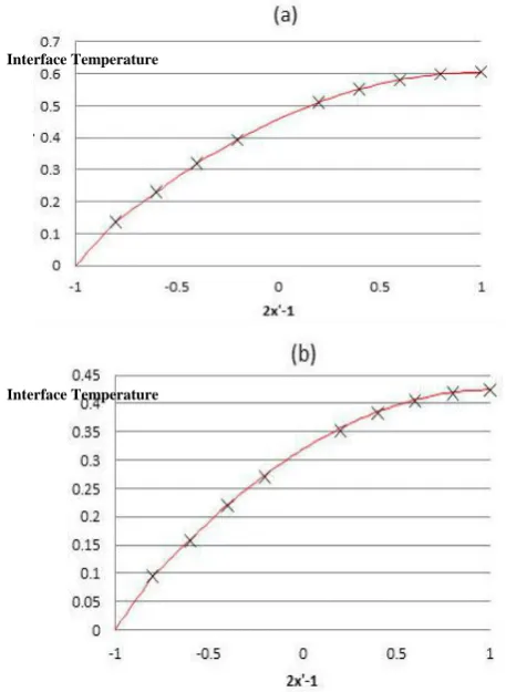
Fig. 3 shows a comparison of the temperature distribution calculated at the interface between the solution obtained by the developed Chebyshev polynomial method and that of the CFD solution, when 1/24 and for the two Reynolds numbers of 1,000 and 500,000. The cubic temperature profile was used for this case, and the two solutions are seen to be in reasonable agreement.

Fig. 3 Temperature at the interface for two Reynolds numbers (a) 1 10 and (b) 5 10 , 1/24. ( Chebyshevshev polynomial solution, CFD)

The errors (differences) between the two solution methods when Re = 500,000 and 1/4 are shown on Fig. 4, and, as can be seen, the differences for this flow are reasonable over most of the heated plate, except near the start where differences in the region of 3.5% were found.

Fig. 4 Errors (differences) between the Chebyshev polynomial and CFD solutions for 5 10 , at 1 24 ⁄ and 1/2.

Fig. 5 shows the results of the temperature calculated at the interface for 1/2. In this case only the quadratic temperature profile was used. It is striking that the temperature distribution for 5 10 is an almost linear profile as calculated by both the CFD and Chebyshev polynomial solutions. Also, as the rise in temperature along the plate surface is so small the temperature distribution could also be approximated to being constant. Differences in the results between the two solution methods are shown on Fig.4 and found to be reasonable except close to the beginning of the plate.

Fig. 5 Temperature at the interface for two Reynolds numbers (a) 1 10 and (b) 5 10 , 1/2. ( Chebyshevshev polynomial solution, CFD)

Interface Temperature

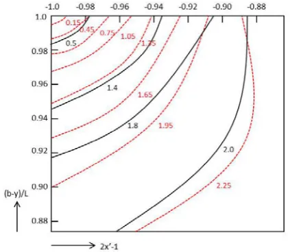
Fig. 6 shows the temperature distribution for the inside of the plate close to its start for the two solution methods. The distribution is given for 1 10 and 1 4⁄ . It can be seen that the temperature field is two-dimensional for both cases. Reasonable agreement was found between the temperature contours for the solution methods.

Fig. 6 Solid temperature distributions comparison for the CFD and Chebyshev polynomial methods for 1 10 and 1 4⁄ .

( CFD, -- Chebyshev polynomial)

VII. CONCLUSIONS

A method using Chebyshev polynomials was developed to calculate the conjugate heat transfer between solid and fluid domains. The results found were encouraging with most calculated using the cubic temperature distribution along the surface. At higher Reynolds numbers and larger plate thicknesses it was concluded that the third-order polynomials can be relaxed to that of second-order or even linear.

REFERENCES

[1] F. K. Tsou, E. M. Sparrow, and R. J. Goldstein, “Flow and

heat transfer in the boundary layer on a continuous moving surface,”

International Journal of Heat and Mass Transfer, vol.10, no. 2, pp.113-256, 1967.

[2] T. Cebeci and P. Bradshaw. Physical and Computational Aspects of Convective Heat Transfer. New York: Springer Verlag, 1984.

[3] S. Kakaç, H. Yűncű, and K. Hijikata (Eds.) Cooling of Electronic Systems. Çesme/Izmir, Turkey, June 21-July, 1993.

[4] W. Khan, J. R. Culham, M. M. Yovanovich, “Optimization of microchannel heat sinks using entropy generation minimization method.” IEEE Transactions of Components and Packaging Technologies, vol. 32, no. 2, pp. 243-251, 2009.

[5] D. Adair and P. G. Tucker, “Efficient modelling of rotating disks and cylinders using a Cartesian grid.” Applied Mathematical Modelling, vol. 21, pp.749-762, 1997.

[6] E. M. F. Elbarbay and N. S. Elgazery, “Chebyshev finite difference method for the effects of variable viscosity and variable thermal conductivity on heat transfer from moving surfaces with radiation.”

International Journal of Thermal Sciences, vol. 43, no. 9, pp. 889-899, 2004.

[7] J. M. Zhao and L. H. Liu, “Least-squares spectral element method for radiative heat transfer in semitransparent media.” Numerical Heat Transfer, Part B, vol. 50, pp. 473-489, 2006.

[8] P. Le Quere and T. A. de Roquefort, “Computation of natural convection in two dimensional cavity with Chebyshev polynomials.”

J. Comp. Phy., vol. 57, pp. 210-228. 1985.

[9] T. G. Sidwell, S. A. Lawson, D. L. Straub, K. H. Casleton, and S. Beer. “Conjugate heat transfer modeling of film-cooled, flat-plate test specimen in a gas turbine aerothermal test facility.” presented at

ASME Turbo 2013: Turbine Technical Conference and Exposition, vol. 3B: Heat Transfer, San Antonio, Texas, USA, June, 2013. [10] J. Batina, S. Blancher, C. Amrauche, M. Batchi, and R. Creff.

Convective Heat Transfer of Unsteady Pulsed Flow in Sinusoidal Constricted Tube. in Convection and Heat Transfer, InTech, 2011. [11] A. S. Dorfman. Conjugate Problems in Convective Heat transfer.

CRC Press, 2010.

[12] T. J. Rivlin,. Chebyshev Polynomials: From Approximation Theory to Algebra and Number Theory. Wiley and Sons, 1990.

[13] M. C. Seiler and F. A. Seiler. Numerical Recipes in C: The Art of Scientific Computing. Cambridge University Press, 1988-1992. [14] S. A. Gbadebo, S. A. M. Said, and M. A. Habib, “Average Nusselt

number correlation in the thermal entrance region of steady and pulsating turbulent pipe flows.” Heat and Mass Transfer, vol. 35, pp.

377-381, 1999.

NOMENCLATURE plate thickness.

local Biot number. average Biot number. heat capacity.

local convective heat transfer coefficient. average convective heat transfer coefficient. thermal conductivity.

′ thermal conductivity ratio. length of the plate. ′ dimensionless length.

local Nusselt number. average Nusselt number. local Peclet number. ′′ heat flow per unit area.

′′ heat flow at the solid-fluid interface.

Re Reynolds number.

temperature.

free-stream temperature. Chebyshev polynomial, ith order. streamwise velocity. ′ dimensionless streamwise velocity.

free-stream velocity. cross-stream velocity. ′ dimensionless cross-stream velocity. streamwise distance. ′ dimensionless streamwise distance. ′′ Chebyshev variable.

solid and cross stream distance.

′ dimensionless solid and cross stream distance.

Greek symbols

ratio ( ⁄ . product ( .

kinematic viscosity.

dimensionless temperature. density.

Subscripts

o free-stream. s solid/interface