The Experimental and Numerical Approch of Two- phase Flows by a Wall Jets on Rough Beds in Open Channel Flow

The Experimental and Numerical Approch of

Two-phase Flows by a Wall Jets on Rough Beds in Open

Channel Flow

Mohamed Ghoma, Khalid Hussin and Simon Tait

Abstract— This paper presents the results of investigations carried out to study the effect of horizontal wall jets on a fixed rough bed in an open channel. The study used both numerical and experimental approaches. The numerical and experimental studies are compared for validation. The main objective of this study is to understand the effect of wall jets on a horizontal fixed rough bed in an open channel.

The experimental study investigated the effect of wall jets on a fixed horizontal bed, with a known roughness in an open channel flume. A sid-looking Acoustic Doppler Velocimetry (ADV) was used to measure the velocity profile of the flow at different flow zones. The wave monitor was used to measure the free surface during the experiments.

Computational fluid dynamics CFD simulations were conducted in a rectangular channel to compare with the laboratory tests using the volume of fluid VOF multiphase method and K- model. The two phase (water and air) was used in this study. Computer simulations for the model were used to predict the fluid horizontal velocity (u) revealing the characteristics of the wall jet over different flow zones (developing, fully developed and recovering zones).

The results showed that the velocity profiles distribution in the stream wise direction in the channel were reasonable. The reverse velocity was close to the wall jet and the maximum reverse velocity was observed near the water surface. Also the results showed that the depression was close to the wall jet.

The agreement between the results obtained from the numerical and the experimental data were reasonable.

Index Terms— VOF method, Two-phase flow, ADV

I. INTRODUCTION

Study of turbulent flows in open channels is considered an important activity in the field of hydraulic engineering. Rivers, canals, drainage channels and sewers are all subject to turbulent flows.

Over decades the study of the phenomenon ofturbulent flow has led to the development of many theories and methods, which have changed thebehaviour of water bodies in favour of sustainable environment and development (Fenton, 2007).Glauert (1956) analysed the wall jet on a horizontal bed. Schwarz and Cosart (1961) estimated the bed shear and Reynolds stresses in a turbulent wall jet by solving the equations of motion for a steady turbulent flow. Rajaratnam (1967) measured the velocity and bed shear stress for plane turbulent wall jets on artificial rough beds using Pitot and

Manuscript received February 06, 2014; revised March 27, 2014.

Mohamed Ghoma, Faculty of Engineering, Al-jabel Al-gharbi University, Gharian, Libya, e-mail: ([email protected]).

Khalid Hussin and Simon Tait with the School of Engineering, Design and Technology, University of Bradford, Bradford, BD7 1DP, UK, e-mails: (k.hussain1, s.tait ) @ Bradford.ac.uk

Preston Tubes. Sinha et al. (1998) presented a three-dimensional numerical model for simulating flow through a river. They included the large-scale bed roughness using a boundary-fitted mesh and also used a two-point wall function approach. The result showed good agreement with the laboratory and measurements. Xingwei and Yee (2003) performed experiments in a laboratory flume with smooth and rough beds. The velocity measurements were conducted using a micro (ADV) and a Laser Doppler Velocimeter (LDV). The results showed a gradual change of the velocity profile as the flow moved from the smoother sand bed to the rough marble bed. The shear velocities are expectedly larger on the marble bed than those on the sand bed. Response of the equivalent roughness height, bed – shear stress, turbulent intensities and Reynolds shear stress were also considered in their analysis. Changes in the velocity fields occurred gradually over a transitional length along the bed for about 5 to 6 times the depth of flow. Halloran, et al. (2005) conducted experiments to investigate the two- phase stratified, wavy flow along with the transition from wavy to slug flow. Computational fluid dynamics CFD simulations were conducted on a similar geometry using the volume of fluid VOF two phase model. Fluent software was used for the simulation. The inlet velocity was uniform at 4 m/s and the height of air in the channel was 10 mm. The outlet was set as a uniform pressure outlet. The standard K- turbulence model was used and a time dependant solution was calculated. Gravitational effects were included and surface tension within a value of 0.072 N/m was specified for the air-water interfaces. A grid of 349888 elements was used to simulate the model. Their results showed that for the wavy flow the steady state numerical results (FLUENT simulations using VOF method) compared with PIV measurements were reasonable. Dey and Sarkarl (2007) presented the Reynolds and boundary shear stresses in submerged jets on horizontal rough boundaries. They measured the flow in submerged jets on horizontal rough boundaries with Doppler velocimeter (ADV). Their results showed that the boundary shear stress increase in longitudinal distance and increases with increase in boundary roughness. The present study considers the effect of wall jets on a rough bed in open channel flow. This case has considerable importance in practice but has not received as much attention as other types of channel flow.

II. EXERIMENTALFACILITYANDPROCEDURE

cross-section. A schematic of the flume is shown in Figure 1. The dimensions of the flume are: 0.20m wide, 0.3m high and 4.05 m long with an adjustable slope. The wall jets openings 10mm. The sidewall of the flume is made of transparent glass to facilitate velocity measurements using Acoustic Doppler velocimetry ADV. The test was carried with fixed rough beds. The experiments were carried out on hydraulically rough bed create using uniformly sized sand.

Flow

Z X

Rough bed

(a)Top view

Inlet T a nk

R o ug h b ed w a ll

T o tail ta nk F lo w

W a ll je t

y

F ro m s um p

(b) Side view

(c) The wall jet facility

Figure 1. A schematic of the experimental setup

A stable wall jet will be created using the constant head. The wall jet test facility is fixed on the bottom of tank shown in figure 1(c). The inlet for the wall jet will be placed 2 m downstream of the channel inlet. The jet velocity is determined by height h, this will be adjusted to change the jet velocity. The jet will be submerged by using a fixed downstream control. The velocity is an equal to the jet discharge velocity. One pump provided the water supply to the header tank with the flow rate controlled by hand-operated valve situated at the inlet. The water discharge was measured by collecting 300 litters of water in a container and recording elapsed time with a stopwatch. The experimental conditions are given in Table I.

Table I. Experimental conditions for fixed bed

III. ACOUSTICDOPPLERVELOCIMETERAND MEASUREMENTS

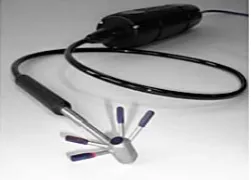
In this present study a side-looking Acoustic Doppler Velocimeter (ADV) was used to measure the effect of horizontal wall jets were on a rough bed in open channel flow. The ADV sensor consists of four acoustic receivers and

a transmitter. The ADV probe is the assembly of the sensor and cable (see Fig 2).

Figure 2. Side-Looking ADV probe

The velocity field for experiment A is measured by the ADV instrument. The hydraulic characteristics of the experiment are given in Table 1. An Acoustic Doppler Velocimeter ADV was used to measure velocity profiles at different streamwise distances. The emitter transducer at the centre generates a short ultrasonic pulse at a fixed carrier frequency that insonifies the water column. The pulses were repeated with a frequency of 100 Hz. In order to obtain the steady time-averaged velocity, a relatively long sampling time was used. The duration of the measurements for every position was set at 2 minutes. The velocity records for each position containing 12000 data points. We calculate the average velocity, , simply by taking the average of the 12000 measurements:

∑ (1)

Where N is the total number of measurements (in this case 12000), and is an individual velocity measurement. The temperature of water in all experiments ranged from 17-26oC.The location of measuring volume is determined by the physical construction of the probe 5 cm from the tip of the probe. The standard measuring volume is a cylinder of water with a diameter 6 mm.

IV. THEWAVEMONITORANDMEASUREMENTS

The free-surface profile was measured using a three probe Churchill Instruments wave monitor. The position of the water surface was measured at different locations and at a frequency of 100 Hz for 3 minutes so that a stable steady value of water depth could be obtained.

V. EXPERIMENTALRESULTS

calibration of the wave monitor. An overall calibration from wave height to output voltage can be performed by noting the change in output voltage when the probe is raised and lowered by a known amount in still water.

Figure 3. Calibration of the wave monitor

The wave monitor works on the principle of measuring the current flowing in a probe which consists of a pair of parallel stainless steel wires. The probe is energised with a high frequency square wave voltage to avoid polarisation effects at the wire surfaces. The wires dip into the water and the current that flows between them is proportional to the depth of immersion. The current is sensed by an electronic circuit providing an output voltage proportional to the instantaneous depth of immersion. The wave monitor was set at scan rate of 100 Hz and the duration of the measurements was set at 3 minutes. The free-surface each point containing 18000 samples. Figure 4. Show that the height of the free surface increases as the velocity inlet increased. Also the depression close to the wall jet increased.

Figure 4. Free surface for Test A and B

VI. MATHEMATICALMODELING

Numerical simulations were carried out using the FLUENT to simulate unsteady jet flow in a 2-dimensional rectangle open channel. For the validation study this model solved using the volume of fluid VOF multiphase method

with RNG k- turbulent model (Yakhot and Orszag, 1986). In the VOF model a single set of momentum equations is shared by the different fluids and the volume fraction of each of the fluids in each computational cell is tracked throughout the domain (FLUENT, 2006). In each control volume, the volume fraction of all phases sum to unity. The volume fraction equation will not be solved for the primary phase; the primary-phase volume fraction will be computed based on the following constraint:

∑ 1 (2)

The fluid is divided into two zones. Water zone and air zone which is separated by a surface tension.

VII. Solution Procedure

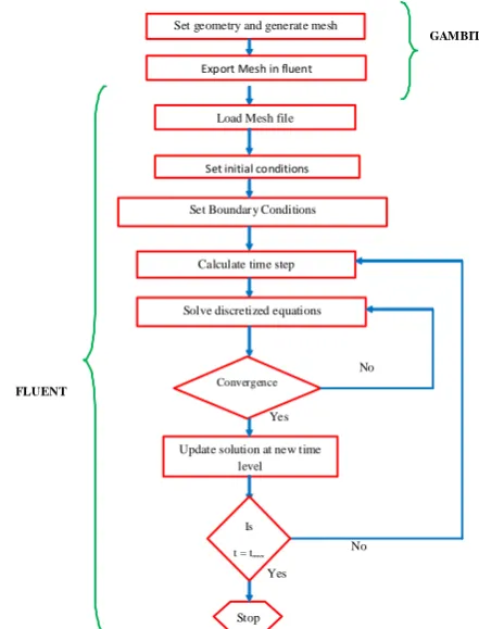
The fluid flow pattern, the velocity profile as the flow moved over the rough bed, the boundary shear stress and the volume fraction contours are determined by solving the model. Figure (6) shows a flowchart of the simulation process from defining the geometry to obtaining the final solution.

Figure 5 - Flow chart describing the solution procedure

VIII. Turbulence Model

The renormalization group (RNG) theory model is commonly used to model channel flows because it performs better than the standard k- model in situation involving complex channel geometry (e.g. Bradbrook et al.,1998).

IX. Boundary and Initial conditions

Inlet boundary condition

Inlet velocity inlet boundary condition was used at the surfaces that have been defined as velocity inlet.

  GAMBIT

No

FLUENT FLUENT

Yes

No

Yes

Set geometry and generate mesh 

Set Boundary Conditions

Export Mesh in fluent 

Load Mesh file

Set initial conditions

Calculate time step

Solve discretized equations

Update solution at new time level Convergence

Stop Is

Outlet boundary condition

At the outlet of the channel pressure outlet boundary condition was applied zero static pressure (gauge) which is equal to the atmospheric pressure was specified at the outlet.

Wall boundary condition

Wall bounder condition was used to all walls. No-slip boundary condition was imposed at the wall.

X. NUMERICALSOLUTIONPROCEDURE

In this study the geometry of the flow zone was generated by GAMBIT for numerical simulation. The full flow was set as two zones that are air zone (top) and water zone (bottom). The equations have been solved using FLUENT. The 2D and unsteady solver was used to solve the flow. The second order upwind scheme was employed for the momentum, volume fraction and turbulent. PISO algorithm is used for pressure velocity coupling. It provides faster convergence for unsteady flow than the standard SIMPLE approach. Six different model properties were monitored by the fluent solver and checked for convergence. The default convergence criteria are 0.01 for all the six properties. Experience has shown that this value is generally not low enough for convergence. There for scaled residuals was decreased to 10-6 for all equations for all variables. The time dependent simulations are performed with time step size of 0.01 s to achieve numerical stability.

XI. NUMERICALRESULTS

Validation

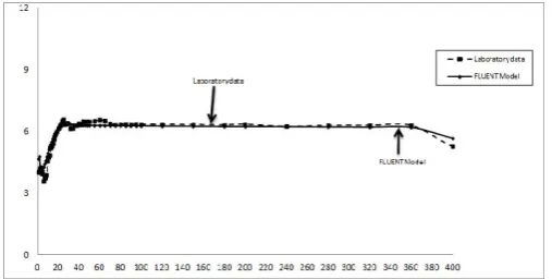
The velocity profiles achieved from VOF method in comparison with the experimental results are shown in figure 7. It is observed that the numerical data match the laboratory results very well. The ADV measurements and the numerical model were taken in the vertical lines at different streamwise distances. Vertical velocity profiles were measured at X [cm] = 4, 6, 10, 15, 20,30,40,50 and 60 downstream of the sluice gate. In the ADV measurements a distance of 1 [mm] is taken between each point in one vertical profile. This was showed the motion of water over the rough beds and how velocity changes with distance.

Figure 6. Time averaged u-velocity profiles of Test A at X [m] = 0.04, 0.06, 0.10, 0.15, 0.20, 0.30, 0.40m and 0.50 from the wall jet

(  Experimental,  Fluent)

was set at 3 minutes. The free-surface each point containing 18000 samples. The height of the free surface increases as the velocity inlet increased. Also the results showed that the depressions close to the wall jet. It is observed that the numerical data match the laboratory results very well.

Figure 7. Comparison of numerical simulated and experimental measured for the free surface

XII. CONCLUSION

In this study, free-surface and velocity distribution on fixed rough bed in open channel flow were obtained both experimentally and numerically. In laboratory test the effect of the rough boundary on the wall jet on the velocity profile was measured by ADV. Using CFD and VOF method simulations of flow were carried out. The experimental and the numerical model both showed that similar pattern of time averaged flow velocities. The results showed that the velocity distribution in the numerical simulations compared reasonably with ADV measurements. Also for the free surface showed that the numerical data match the laboratory results very well.

NOMENCLATURE

Fr Froud No., Fr = U/ hw The tail water depth (m)

X The distance from the inlet (m) d50 The median diameter of sand (m)

Q discharge (m3/s) Ujet The initial jet velocity (m/s)

hjet The inlet opening of sluice gate (m) wjet The wide of the jet (m)

REFERENCES

[1] Fentonn. J (2007). “Open Channel Hydraulics,” Lectures notes. [2] Glauert M B. 1956., “The wall jet,” J. Flued Mech. 1, 625-643. [3] Schwarz W. H., Cosart, W.P., 1961. “The two-dimensional turbulent

wall-jet”. Journal of Fluid Mechanics 10, 48- 495.

[4] Rajaratnam N. And Subramanya K. (1967). “Flow immediately below submerged sluice gate”. Proc. ASCE. HY4.P .57-77.

[5] Sinha SK, Sotiropoulos F and Odgaarrd AJ.(1998). “Three dimensional numerical model for river flow through natural rivers”. J Hydr Res; 124(1):13-24.

[6] Chen, X. and Chiew, Y. M. (2003). “Response of Velocity and Turbulence to Sudden Change of Bed Roughness in Open- Channel Flow.” J.Hydr. Engng., ASCE, 129, 35-43.

[7] O Halloran. P, Mohammad. B. H. Hosni and J. Eckels. Steven (2005).“Experimental Measurements and Numerical Simulation of Two-Phase Stratified, Wavy and Slug Flow in a Narrow Rectangular Channel.” ASME Fluids Eng Summer Conference.

[8] Subhasish Dey and ArindamSarkar.(2007)“Computation of Reynolds and boundary shear stress in submerged jets on rough boundary,”. J Hydraulic Research, ELSEVIER, 110-117.

[9] Yakhot, V., and Orszag, S.A. (1986). “Renormalization Group Analysis of Turbulence,”. I. Basic Theory. Journal of Scientific Computation, 1, 1, 1-51.

[10] Apsley, D. (2003). “CFD simulation of two and three dimensional free surface flow,”. International Journal of Numerical Methods in Fluids, 42, p.465-491.

[11] A. Nasser and Mostaghimi. J. (2002). “An Introduction to Computational Fluid Dynamics,” Jamal Saleh,ed. Fluid Flow Handbook,24.1.

[12] Chiu, C., (1989). “Velocity Distribution in Open Channel Flow,” J.Hydr. Div., ASCE, 115(5), pp. 576-594.

[13] Dey, S and Lambert, M. F. (2005). “Reynolds Stress and Bed Shear in Nonuniform-unsteady Open Channel Flow,” J.Hydr Engng., ASCE, 131, 610-614.

[14] Dey, S and Sarkar, A. (2006). “Response of Velocity and Turbulence in Submerged Wall Jets to abrupt Changes From ,Smooth to Rough Beds and its Application to Scour Downstream of an Apron,”. J. Fluid Mech, Vol. 556, pp. 387- 419.

[15] Ead, S. A., and Rajaratnam, N. (2004). “Plane Turbulent Wall Jets on Rough Boundaries with Limited Tailwater,”. J.Eng. Mech., ASCE, 130, 1245-1250.

[16] O Halloran. P, Mohammad. B. H. Hosni and J. Eckels. Steven (2005). “Experimental Measurements and Numerical Simulations of Two-Phase Stratified, Wavy and Slug Flow in a Narrow Rectangular Channel,” ASME Fluids Eng Summer Conference.

[17] Razmi, Firoozabadi and Goodarz (2008). “Experimental and Numerical Approach to Enlargement of Performance of Primary SettlingTanks,” Journal of Applied Fluid Mechanics, Vol, 2, pp.01-12