Abstract—This paper develops an integrated inventory model consisting of single-vendor and single-buyer system. The demand in buyer side is deterministic and the production process is imperfect and produces a certain number of defective items. The delivery within a single production batch from vendor to buyer is increasing by a fixed factor. After the delivery arrives at the buyer, an inspection process is conducted. The inspection process in not perfect. Errors may occur when the inspector is misclassifies a non-defective item as defective ne, or incorrectly classifies a defective item as non-defective. This model provides an optimal solution for the expected integrated total annual cost of the vendor and the buyer. The result from numerical examples shows that the integrated model will result in lower joint total cost in comparison with the equal-sized policy.
Keywords—Integrated inventory model, Vendor-buyer system, Unequal size, Imperfect quality, Inspection errors
I. INTRODUCTION
ITH the growing business in nowadays, firms have been attempting to achieve greater performance in their supply chain. Since improving supply chain was considered to be the key factor in managing modern business, many firms realized that the best strategies in managing inventories across the supply chain can be more efficiently achieved through better cooperation and better integration with their supply chain partners.
The integrated inventory management model in the supply chain has received a great deal of attention since more than three decades ago. Since Goyal [1] introduced the integrated inventory model consisting of a vendor and a buyer, many researchers have developed the models under various cases, such as [2], [3], [4], [5], [6], [7], [8], [9].
Further, Goyal [10] developed a model of vendor-buyer with unequal-sized shipment. Some researchers, including [11], [12], [13], [14], [15] proposed vendor-buyer model under unequal-sized shipment and proved that the proposed policy gives an impressive cost reduction in comparison to equal-sized policy. The above mentioned papers assumed that the product produced by the vendor is always in perfect
*Manuscript received January 09, 2014; revised January 27, 2014. Imanuel Prasetyo Widianto is student in the Department of Industrial Engineering Sebelas Maret University, Jl. Ir Sutami 36A, Surakarta, 57126, Indonesia (corresponding author, phone: +62-856-2500315; fax: +62-271-632110; e-mail: imanuelprasetyo@gmail.com).
Wakhid Ahmad Jauhari is a researcher in the Production System Laboratory, Department of Industrial Engineering, Sebelas Maret University, Jl. Ir Sutami No. 36A, Surakarta, Indonesia (e-mail:
wachid_aj@yahoo.com).
Cucuk Nur Rosyidi is a researcher in the Production System Laboratory, Department of Industrial Engineering, Sebelas Maret University, Jl. Ir Sutami No. 36A, Surakarta, Indonesia (e-mail: cucuknur@gmail.com).
quality. However, in real situation, the production process may produce a certain number of defective items. Porteus [16] was among the first researchers who introduced an EPQ model considering defective items and showed a significant relationship between quality and lot size.
Therefore, some researchers are interested in developing inventory model considering imperfect quality. Salameh and Jaber [17] developed an EOQ model assuming that the lot contains a random proportion of defective items. The model assumed that there is no error caused by human in the inspection process. Then, Raouf et al. [18] studied human errors in inspection. Yoo et al. [19] proposed a model that considered both imperfect production and two-way imperfect inspection. The model considered the situation in which the inspector may incorrectly classify a non-defective item as defective (Type I inspection error), or incorrectly classify a defective item as non-defective (Type II inspection error). Lin [20] developed a model for simple supply chain system based on [19] and assumed that both Type I and Type II inspection errors are known constants. Hsu and Hsu [21] then developed an integrated vendor-buyer inventory model for items with imperfect quality and inspection errors. This model assumes that the defective items are sold to a secondary market at a discounted price. Furthermore, Darwish et al. [22] examined the effect of imperfect quality in vendor-buyer system under vendor managed inventory model.
Most of above models, studied vendor-buyer model with defective items and equal-sized shipment. Pamudji et al. [23] developed a model with unequal-sized shipment policy and defective items and also showed that the proposed model can reduce the total cost significantly compared to equal-sized shipment. In this paper, we propose an integrated inventory model for single-vendor single-buyer which considers unequal-sized shipment, defective items, and inspection errors for vendor-buyer system.
II. ASSUMPTIONS AND NOTATIONS
2.1
AssumptionsThe assumptions used in this paper are:
1) The demand rate is known, constant, and continuous. 2) The lead time is zero.
3) Demand is deterministic.
4) Backorder and shortage are not allowed. 5) Production rate is greater than the demand rate.
6) Product lots which are sent from the vendor to the buyer contain defective items with defect rate of γ.
7) The inspection process is imperfect and the probability of classifying a non-defective as defective is e1.
8) The probability of classifying a defective as
non-Cooperative Vendor-Buyer Inventory Model
with Imperfect Quality and Inspection Errors
Imanuel Prasetyo Widianto, Wakhid Ahmad Jauhari, Cucuk Nur Rosyidi
defective is e2.
9) The buyer returns all items classified as defective. 10) The items those returned from the costumer to the
vendor at the end of the 100% screening process will be given a full price refund from the vendor.
11) The vendor incurs a cost of cw for each defective item.
12) The vendor will sell the returned items at a discounted price to a secondary market. Therefore, cr is the
difference between the regular and the discounted price. 13) Costumer who buys the defective items will detect the quality problem and return them to the buyer and received a good item for replace. Both the vendor and the buyer incur a post-sale failure cost for the items returned from the market.
2.2
Notations D : Demand rateP : Production rate
Q : The first shipment size of each batch in early production lot
F : Transportation cost per shipment (including the shipment of Q units from the vendor to the buyer and the returned items from the buyer to the vendor)
Sb : Ordering cost per order for the buyer
Sv : Setup cost per production run for the vendor
n : The number of shipments per batch production run, a positive integer
λ : The increasing rate of delivery lot size
γ : The probability that an item produced is defective
x : Inspection rate
ci : Inspection cost per unit for buyer
cw : Unit cost for producing defective items for
vendor
cab : Post-sale defective items cost for buyer
cav : Post-sale defective items cost for vendor
cr : The cost of rejecting a non-defective item
Hv : The holding cost per unit per year for the vendor
Hb : The holding cost per unit per year for the buyer
JTC : Joint total cost
B1 : The number of items that are classified as
defective in each delivery of Q units
B2 : The number of items that are returned from the
market in each delivery of Q units
e1 : The probability of a Type I inspection error
(classifying a non-defective item as defective)
e2 : The probability of a Type II inspection error
(classifying a defective item as non-defective) III. MODEL DEVELOPMENT
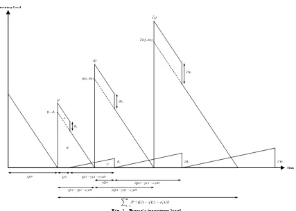
Here, we discuss about a single item in a single-vendor single-buyer inventory problem with unequal-sized shipment, defective items, and inspection errors. The terminology for the proposed unequal-sized policy is adopted from [23] and the production rate is greater than the demand rate (P>D). We assume that the production rate is greater than the demand rate (P>D). The first shipment is conducted with a lot size of Q. Then, the next shipments are done with a lot size of λn-1Q. λ is the growth factor which is
determined between 1 and P/D. Each lot contains a probability of defective items γ and after receiving the lot from the vendor, the buyer performs the inspection process. The inspection process is not perfect. While inspecting the items, errors may occur because of human activity. The inspector may misclassify non-defective items as defective with probability e1, or misclassify defective items as
[image:2.595.84.511.460.765.2]non-defective. The defective item which are found by inspector in buyer’s inspection process and each defective item that returned from the market to the vendor as a single batch at
Fig. 1. Buyer’s inventory level
Inventory Level
Time
B2 λB2 λ
2
B2
B1
λB1
λ2B 1
Q - B1
λ(Q - B1)
λ2(Q - B
1)
Q
λQ
λ2
Q
Q/P Q/x Q(1 – γ)(1 – e1)/D
λQ/x A
B
C
Q(1 – γ)(1 – e1)/D λQ(1 – γ)(1 – e1)/D
the end of the inspection process will receive a full price refund from the vendor as a warranty. The vendor will incurs a cost cw from each defective item and incurs a cost
of cr for each non-defective items classified as defective.
The vendor will incur a cost cw from each defective item and
incur a cost of cr for each non-defective item classified as
defective. The buyer incurs a post-sale cost cabper unit item
returned from the market while the vendor incurs cavper unit
item.
The objective function of this model is to minimize the joint total cost per unit time (TC) that consists of the buyer’s total inventory cost (TCB) and the vendor’s total inventory
cost (TCV)
3.1
The Buyer’s Cost FormulatonThe buyer’s total inventory cost consists of ordering cost (OCb), delivery cost (FC), inspection cost (IC), post-sale
failure cost (PC), and the buyer’s holding cost (HCb).
Fig. 1 shows the buyer’s inventory level for each ordering cycle. By definition, B1 is calculated as follows
𝐵1= 𝑄(1 − 𝛾)𝑒1+ 𝑄𝛾(1 − 𝑒2) (1)
𝐵2= 𝑄𝛾𝑒2 (2)
The production batch can be calculated as follows ∑𝑛 𝜆𝑖−1
𝑖=1 (𝑄 − 𝐵1− 𝐵2) =𝑄(1−𝛾)(1−𝑒1)(𝜆
𝑛−1)
(𝜆−1) (3)
Hence, a number of production cycle can be formulated by dividing the demand (D) with (3):
𝐷
𝑄(1−𝛾)(1−𝑒1)(𝜆𝑛−1)/(𝜆−1) (4)
The total defective items per production cycle can be formulated by considering the rectangle A in Fig. 1, that is 𝐻𝐶𝑏1=𝑄
2(𝜆2𝑛−1)(1−𝛾)𝑒1
𝑥(𝜆2−1) +
𝑄2𝛾(𝜆2𝑛−1)(1−𝑒2)
𝑥(𝜆2−1) (5)
Meanwhile, the total inventory for buyer per production run can be calculated by considering the triangle B in Fig. 1 and is formulated by
𝐻𝐶𝑏2=(𝜆
2𝑛−1)
(𝜆2−1) .
𝑄2[1−(1−𝛾)𝑒1+𝛾(1−𝑒2)](1−𝛾)(1−𝑒1)
2𝐷 (6)
Thus, by considering the triangle C in Fig. 1, the total item items returned from the market in one production cycle is given as follows
𝐻𝐶𝑏3=(𝜆
2𝑛−1)
(𝜆2−1) .
𝑄2𝛾𝑒2(1−𝛾)(1−𝑒1)
2𝐷 (7)
Further, the holding cost for the buyer in one production cycle can be found by adding (5) and (6) into (7), that is 𝐻𝐶𝑏 = 𝐻𝑏𝑄𝐷 {(𝜆
2𝑛𝑒1−𝜆2𝑛𝛾𝑒1−𝑒1+𝛾𝑒1)+(𝜆2𝑛𝛾−𝜆2𝑛𝛾𝑒2−𝛾+𝛾𝑒2)
𝑥(𝜆+1)(1−𝛾)(1−𝑒1)(𝜆𝑛−1) }
+𝐻𝑏𝑄𝛾𝑒2(𝜆𝑛+1)
2(𝜆+1) +
𝐻𝑏𝑄𝑒1(1−𝑒1+𝛾𝑒1+𝛾−𝛾𝑒2)(𝜆𝑛+1)
(𝜆+1) (8)
After adding the warranty, ordering, delivery, inspection, and post-sale failure cost for each production run, the buyer’s total cost is given by
𝐸𝑇𝐶𝑏(𝑛, 𝑄, 𝜆) =
(𝑆𝑏+ 𝑛𝐹)𝑄(1−𝛾)(1−𝑒𝐷(𝜆−1)
1)(𝜆𝑛−1)+(𝑐𝑖+ 𝑐𝑎𝑏𝛾𝑒2)
𝐷
(1−𝛾)(1−𝑒1)
+𝐻𝑏𝑄𝐷 {(𝜆
2𝑛𝑒1−𝜆2𝑛𝛾𝑒1−𝑒1+𝛾𝑒1)+(𝜆2𝑛𝛾−𝜆2𝑛𝛾𝑒2−𝛾+𝛾𝑒2)
𝑥(𝜆+1)(1−𝛾)(1−𝑒1)(𝜆𝑛−1) }
+𝐻𝑏𝑄𝛾𝑒2(𝜆𝑛+1)
2(𝜆+1) +
𝐻𝑏𝑄𝑒1(1−𝑒1+𝛾𝑒1+𝛾−𝛾𝑒2)(𝜆𝑛+1)
(𝜆+1) (9)
3.2
The Vendor’s Cost FormulationThe vendor’s total inventory cost consist of setup cost, warranty cost, Type I and Type II errors cost, and holding cost for the vendor. The holding cost for vendor is based on
[23], that is 𝐵𝑆𝑣 =
𝐻𝑣{𝐷𝑄𝑃 +(𝑃−𝐷)𝑄(𝜆
𝑛−1)
2𝑃(𝜆−1) −
𝑄(𝜆𝑛+1)
2(𝜆+1) (1 − 𝛾)
2−𝑄𝛾𝐷(𝜆𝑛+1)
𝑥(𝜆+1) } (10)
The total cost for the vendor can be formulated by adding the setup cost, warranty cost, Type I and Type II errors costs into (10). The formulation is as follows
𝐸𝑇𝐶𝑣(𝑛, 𝑄, 𝜆) =
𝑆𝑉𝑄(1−𝛾)(1−𝑒𝐷(𝜆−1)
1)(𝜆𝑛−1)+ (𝑐𝑤𝛾 + 𝑐𝑎𝑣𝛾𝑒2)
𝐷
(1−𝛾)(1−𝑒1)+
𝑐𝑟𝐷𝑒1
(1−𝑒1)
+ 𝐻𝑣{𝐷𝑄𝑃 +(𝑃−𝐷)𝑄(𝜆
𝑛−1)
2𝑃(𝜆−1) −
𝑄(𝜆𝑛+1)
2(𝜆+1) (1 − 𝛾)
2−𝑄𝛾𝐷(𝜆𝑛+1)
𝑥(𝜆+1) } (11)
3.3
Joint Total Cost FormulationThe joint total cost for vendor-buyer is formulated by summing the buyer cost (9) and the vendor cost (11). The formulation is given as follows
𝐽𝑇𝐶(𝑛, 𝑄, 𝜆) =
(𝑆𝑣+𝑆𝑏+𝑛𝐹)𝐷(𝜆−1)
𝑄(1−𝛾)(1−𝑒1)(𝜆𝑛−1)+
(𝑐𝑤𝛾+𝑐𝑖+𝑐𝑎𝑏𝛾𝑒2+𝑐𝑎𝑣𝛾𝑒2)𝐷
(1−𝛾)(1−𝑒1) +
𝑐𝑟𝐷𝑒1
(1−𝑒1)
+ 𝐻𝑣{𝐷𝑄𝑃 +(𝑃−𝐷)𝑄(𝜆
𝑛−1)
2𝑃(𝜆−1) −
𝑄(𝜆𝑛+1)
2(𝜆+1) (1 − 𝛾)
2−𝑄𝛾𝐷(𝜆𝑛+1)
𝑥(𝜆+1) }
+𝐻𝑏𝑄𝐷 {(𝜆
2𝑛𝑒1−𝜆2𝑛𝛾𝑒1−𝑒1+𝛾𝑒1)+(𝜆2𝑛𝛾−𝜆2𝑛𝛾𝑒2−𝛾+𝛾𝑒2)
𝑥(𝜆+1)(1−𝛾)(1−𝑒1)(𝜆𝑛−1) }
+𝐻𝑏𝑄𝛾𝑒2(𝜆𝑛+1)
2(𝜆+1) +
𝐻𝑏𝑄𝑒1(1−𝑒1+𝛾𝑒1+𝛾−𝛾𝑒2)(𝜆𝑛+1)
(𝜆+1) (13)
3.4
Solution MethodologyIn this section, we develop a solution methodology to find the optimal solution of the model. Taking the first partial derivative of ETC(n, Q, λ) with respect to Q, we obtain
𝜕𝐽𝑇𝐶(𝑛,𝑄,𝜆)
𝜕𝑄 =
−(𝑆𝑣𝐷+𝑆𝑏𝐷+𝑛𝐹𝐷)(𝜆−1)
𝑄2(1−𝛾)(1−𝑒1)(𝜆𝑛−1)+
𝐻𝑣𝐷
𝑃 +
𝐻𝑣(𝑃−𝐷)(𝜆𝑛−1)
2𝑃(𝜆−1) −
𝐻𝑣(𝜆𝑛+1)(1−𝛾)2
2(𝜆+1)
+𝐻𝑏𝐷 {(𝜆
2𝑛𝑒1−𝜆2𝑛𝛾𝑒1−𝑒1+𝛾𝑒1)+(𝜆2𝑛𝛾−𝜆2𝑛𝛾𝑒2−𝛾+𝛾𝑒2)
𝑥(𝜆+1)(1−𝛾)(1−𝑒1)(𝜆𝑛−1) }
−𝐻𝑣𝛾𝐷(𝜆𝑛+1)
𝑥(𝜆+1) +
𝐻𝑏𝛾𝑒2(𝜆𝑛+1)
2(𝜆+1) +
𝐻𝑏𝑒1(1−𝑒1+𝛾𝑒1+𝛾−𝛾𝑒2)(𝜆𝑛+1)
(𝜆+1) (14)
Taking the second derivative of ETC(n, Q, λ) with respect to Q we will find
𝜕𝐽𝑇𝐶(𝑛,𝑄,𝜆)
𝜕𝑄2 =
2(𝑆𝑣𝐷+𝑆𝑏𝐷+𝑛𝐹𝐷)(𝜆−1)
𝑄3(1−𝛾)(1−𝑒1)(𝜆𝑛−1) (15)
Clearly, it can be seen in (15) that 𝜕𝐽𝑇𝐶(𝑛,𝑄,𝜆)𝜕𝑄2 > 0 with fixed value of n and λ. It implies that the joint total cost for vendor-buyer is a convex function, hence there is exist the optimal value of shipment quantity that minimizes (13). By setting (14) equals to zero, the optimal shipment quantity is given by
𝑄∗= √(𝑆𝑣𝐷+𝑆𝑏𝐷+𝑛𝐹𝐷)(𝜆−1)(1−𝛾)(1−𝑒1)(𝜆𝑛−1)
𝑌 +𝑍 (16)
with 𝑌 =𝐻𝑣𝐷
𝑃 +
𝐻𝑣(𝑃−𝐷)(𝜆𝑛−1)
2𝑃(𝜆−1) −
𝐻𝑣(𝜆𝑛+1)(1−𝛾)2
2(𝜆+1) −
𝐻𝑣𝛾𝐷(𝜆𝑛+1)
𝑥(𝜆+1)
and 𝑍 = 𝐻𝑏𝐷 {(𝜆
2𝑛𝑒1−𝜆2𝑛𝛾𝑒1−𝑒1+𝛾𝑒1)+(𝜆2𝑛𝛾−𝜆2𝑛𝛾𝑒2−𝛾+𝛾𝑒2)
𝑥(𝜆+1)(1−𝛾)(1−𝑒1)(𝜆𝑛−1) }
+𝐻𝑏𝛾𝑒2(𝜆𝑛+1)
2(𝜆+1) +
𝐻𝑏𝑒1(1−𝑒1+𝛾𝑒1+𝛾−𝛾𝑒2)(𝜆𝑛+1)
IV. NUMERICAL EXAMPLES
In this paper, we consider an example given by Hsu and Hsu [21], where:
P = 160.000 units/year
D = 50.000 units/year
x = 175.200 units/year
Sv = $300/production run
Sb = $100/order
Hv = $2/unit/year
Hb = $5/unit/year
F = $25/delivery
ci = $0,5/unit
cw = $50/unit
cr = $100/unit
cab = $200/unit
cav = $300/unit
If the defective percentage and inspections errors follow a uniform with
𝑓(𝛾) = {
1
𝛽, 0 ≤ 𝛾 ≤ 𝛽
0, 𝑜𝑡ℎ𝑒𝑟𝑤𝑖𝑠𝑒 𝑓(𝑒1) = {
1
𝜆, 0 ≤ 𝑒1≤ 𝜆
0, 𝑜𝑡ℎ𝑒𝑟𝑤𝑖𝑠𝑒 𝑓(𝑒2) = {
1
𝜂, 0 ≤ 𝑒2≤ 𝜂
0, 𝑜𝑡ℎ𝑒𝑟𝑤𝑖𝑠𝑒 Then we have
𝐸[𝛾] = ∫ 𝛾𝑓(𝛾)𝑑𝛾 =0𝛽 ∫0𝛽𝛽𝛾𝑑𝛾 =𝛽2 , 𝐸[𝛾2] = ∫ 𝛾𝛽 2𝑓(𝛾)𝑑𝛾 =
0 ∫
𝛾2
𝛽 𝑑𝛾 =
𝛽 0
𝛽2
3 ,
𝐸[𝑒1] =𝜆2, 𝐸[𝑒12] =𝜆
2
3, and [𝑒2] = 𝜂
2 . Specifically, if 𝛽 =
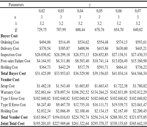
𝜆 = 𝜂 = 0,04, the impact of of defective rate on proposed model can be seen in table 1.
The optimal solution from Hsu and Hsu [21] policy is to manufacture in batches (Q*) of 791 units with n = 7, and the minimum total cost is $201.358,50. Using our proposed model, the optimal solutions from the above problem are Q* = 1.101,39, n = 3 with the shipments sizes 2.335,19 units, 4.670,38 units, and 7.005,57 units. For the minimum total cost in the proposed model is $195.201,03.
Table I gives the illustration of the effect of the changes in defective rate on proposed model. From Table I, it can be seen that the increasing of defective rate will affect the total buyer cost, total vendor cost, and joint total cost. For the vendor, the increasing number of defective items gives significant impact to post-sales failure cost.
V. CONCLUSION
In this paper, we develop a single-vendor single-buyer inventory model for single product considering unequal-sized shipment under deterministic demand, imperfect quality, and inspection errors. The joint total cost of the vendor and buyer is derived and a solution procedure is provided to find the optimal solution that can minimize the joint total cost. The result from numerical example shows that the model can give benefit to both parties. In addition, the joint total cost decreases when the defect rate decreases.
REFERENCES
[1] Goyal, S.K. “An Integrated Inventory Model for A Single Supplier – Single Customer Problem” International Journal of Production
Research., Vol. 15, 1976, pp.107-111.
[2] Banerjee, A. “A joint economic-lot-size model for purchaser and vendor”, Decision Sciences, Vol. 17, No. 3, 1986, pp. 292-311. [3] Goyal, S.K. “A Joint Economic-Lot-Size Model for Purchaser and
Vendor: A Comment”, Decision Sciences, Vol. 19, 1988, pp. 236-241.
[4] Goyal, S.K. and Gupta, Y.P. “Integrated inventory models: the buyer-vendor Coordination”, European Journal of Operational Research, Vol. 41, 1989, pp. 261-269.
[5] Jauhari, W.A., Pujawan, I.N., Wiratno. S.E. and Priyandari, Y. “Integrated inventory model for single-vendor single-buyer with probabilistic demand”, International Journal of Operational
Research, Vol. 11, No. 2, 2011, pp. 160-178.
[6] Gupta, O.K., Shah, N.H., Patel, A., R. “An integrated deteriorating inventory model with permissible delay in payments and price sensitive stock-dependent demand”, International Journal of
Operational Research”, Vol. 11, No. 4, 2011, pp. 452-442.
[7] Madhavi, N., Rao, K.S., Lakshminarayana, J. “Optimal pricing policies of an inventory model for deteriorating items with discounts”,
International Journal of Operational Research, Vol. 12, No. 4, 2011,
pp. 464-480.
[8] Jauhari, W.A. “Integrated inventory model for three-layer supply chain with stochastic demand”, International Journal of Operational
Research, Vol. 13, No. 3, 2012, pp. 295-317.
[9] Gupta, V. and Singh, S.R. “An Integrated inventory model with fuzzy variables, three-parameter Weibull deterioration and variable holding cost under inflation”, International Journal of Operational Research, Vol. 18, No. 4, 2013, pp. 434-451.
[10] Goyal, S.K. “A one-vendor multi-buyer integrated production inventory model: A comment”, European Journal of Operational
Research, Vol. 82, 1995, pp. 209-210.
[11] Hill, R.M. “The optimal production and shipment policy for the single-vendor single-buyer integrated production-inventory problem”,
International Journal of Production Research, Vol. 37, 1999, pp.
2463-2475.
[12] Hoque, M.A. and Goyal, S.K. “An optimal policy for a single-vendor single-buyer integrated production-inventory system with capacity constraint of the transport equipment”, International Journal of
Production Economics, Vol. 65, 2000, pp. 305-315.
[13] Zhou, Y.W. and Wang, S.D. “Optimal production and shipment models for a single-vendor-single-buyer integrated system”,
European Journal of Operational Research, Vol. 180, 2007, pp.
309-328.
[14] Hill, R.M., and Omar, M. “Another look at the vendor single-buyer integrated production-inventory problem”, International
Journal of Production Research, Vol. 44, 2006, pp. 791-800.
[15] Giri, B.C. and Roy, B. “A vendor-buyer integrated production-inventory model with quantity discount and unequal sized shipment”,
International Journal of Operational Research, Vol. 16, No. 1, 2013,
pp. 1-13. TABLEI
THE IMPACT OF DEFECTIVE RATE ON MODEL
Parameters
0,02 0,03 0,04 0,05 0,06 0,07
n 3 3 3 3 3 3
λ 3,2 3,2 3,2 3,2 3,2 3,2
Q 729,75 707,99 688,44 670,76 654,70 640,02
Buyer Cost
Ordering Cost $494,06 $514,49 $534,62 $554,48 $574,13 $593,61 Delivery Cost $370,54 $385,87 $400,96 $415,86 $430,60 $445,21 Inspection Cost $26.030,82 $26.299,18 $26.573,13 $26.852,85 $27.138,51 $27.430,33 Post-sales Failure Cost $4.164,93 $6.311,80 $8.503,40 $10.741,14 $13.026,49 $15.360,98 Holding Cost $364,73 $442,29 $517,79 $591,71 $664,41 $736,22 Total Buyer Cost $31.425,09 $33.953,63 $36.529,90 $39.156,03 $41.834,14 $44.566,34 Vendor Cost
Setup Cost $1.482,18 $1.543,48 $1.603,85 $1.663,43 $1.722,38 $1.780,82 Warranty Cost $52.061,64 $78.897,54 $106.292,52 $134.264,23 $162.831,09 $192.012,29 Type I Error Cost $102.040,82 $102.040,82 $102.040,82 $102.040,82 $102.040,82 $102.040,82 Type II Error Cost $6.247,40 $9.467,70 $12.755,10 $16.111,71 $19.539,73 $23.041,47 Holding Cost $2.032,34 $2.066,49 $2.100,46 $2.134,15 $2.167,49 $2.200,45 Total Vendor Cost $163.864,37 $194.016,03 $224.792,74 $256.214,34 $288.301,52 $321.075,85 Joint Total Cost $195.201,03 $227.969,66 $261.322,64 $295.370,37 $330.135,65 $365.642,19
[image:4.595.49.289.477.685.2][16] Porteus, E.L. “Optimal lot sizing, process quality improvement and setup cost reduction. Operations Research, Vol. 34, 1986, pp. 137-144.
[17] Salameh, M.K. and Jaber, M.Y. “Economic production quantity model for items with imperfect quality”, International Journal of
Production Economics, Vol. 64, No. 1, 2000, pp. 59-64.
[18] Raouf, A., Jain, J.K., and Sathe, P.T. “A cost-minimization model for multicharateristic component inspection”, HE Transactions, Vol. 15, 1983, pp. 187-194.
[19] Yoo, S.H., Kim, D., and Park, M.S. “Economic production quantity model with imperfect-quality items, two-way imperfect inspection and sales return”, International Journal of Production Economics, Vol. 121, 2009, pp. 255-265.
[20] Lin, T.Y. “Optimal policy for a simple supply chain system with defective items and returned cost under screening errors”, Journal of
the Operations Research Society of Japan, Vol. 52, 2009, pp.
307-320.
[21] Hsu, J.T. and Hsu, L.F. “An integrated single-vendor single-buyer production-inventory model for items with imperfect quality and inspection errors”, International Journal of Industrial Engineering
Computations, Vol. 3, 2012, pp. 703-720.
[22] Darwish, M.A., Odah, O.M, Goyal, S.K. “Vendor-managed inventory models for items with imperfect quality”, International Journal of
Operational Research, Vol. 18, No. 4, 2013, pp. 401-433.