Optimum structures of digital controllers in sampled data systems: a roundoff noise analysis

Optimum structures of digital controllers in

sampled-data systems: a roundoff noise analysis

G . Li, J. Wu, S. Chen and K.Y. Zhao

Abstract: The effect of roundoff noise in a digital controller is analysed for a sampled-data system in which the digital controller is implemented in a state-space realisation. A new measure, called averaged roundoff noise gain, is derived. Unlike the traditionally used measure, where the analysis is performed based on an equivalent digital control system, this newly defined averaged roundoff noise gain allows one to take consideration of the inter-sample behaviour. It is shown that this measure is a function of the state-space realisation. Noting the fact that the state-space realisations of a digital controller are not unique, the problem of optimum controller structure is to identify those realisations that minimise the averaged roundoff noise gain subject to the 12-scaling constraint which is for preventing the signals in the controller from overflow. An analytical solution to the problem is presented and a design example is given. Both theoretical analysis and simulation results show that the optimum controller realisations obtained with the proposed approach are superior to those obtained with the traditional analysis based on a digital control system.

1 Introduction

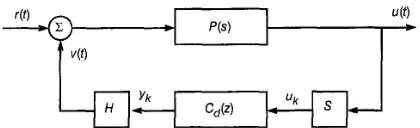
A sampled-data system (see Fig. 1) consists of a continuous-time plant P(s) and a sampled-data controller which is composed of a sampler (A/D converter) S, the digital controller C,(z) to be designed and a hold (D/A converter) H. A digital controller is usually obtained by one of the following two ways: the first one is to design the controller in the continuous-time domain and then perform a digital implementation of the controller, while the second

is to design the digital controller based on a discretised model of the plant. The designed digital controller has to be implemented with a digital device such as a digital control processor. Due to the finite word length (FWL) effects, the actually implemented controller is different from the designed one. Therefore, the actual performance

of the system may be very different from the desired one. Generally speaking, there are two types of FWL errors in the digital controller. The first is perturbation of controller parameters implemented with FWL while the second is the rounding errors that occur in arithmetic operations. Typi-

0 IEE, 2002

TEE Proceedings online no. 20020397

DOI: IO. 1049/ip-cta:20020397

Paper first received 15th November 2000 and in revised forin 8th March 2002

G. Li is with the School o f Electrical and Electronic Engineering, Nanyang Technological University, Singapore 639798

J. Wu is with the National Key Laboratory o f lndustrial Control Technology, Institute o f Advanced Process Control, Zhejiang University, Hangzhou, 3 10027, People’s Republic o f China

S. Chen is with the Department of Electronics and Computer Science, University of Southampton, Highfield, Southampton SO I7 lBJ, UK K.Y. Zhao is with the Institute of Electrical and Control Engineering, Qingdao University, People’s Republic o f China

IEE Proc.-Cantrol Theory Appl., Vul. 149. No. 3, 2002

cally, effects of these two types of errors are investigated separately.

The effects of the first type of FWL errors are classically studied with a transfer function sensitivity measure. In [ 1, 21, the analysis was performed based on the discrete-time counterpart of the sampled-data system. The correspond- ing sensitivity measure does not take the inter-sample behaviour into account. To overcoine this, Madievski

et al. [3] derived a sensitivity measure based on a hybrid operator (transfer function) of the sampled-data system. The corresponding optimal realisation problem was made tractable with a two-step procedure: very fast sampling at a multiple of the sampling frequency followed by ‘blocking’ or ‘lifting’ to achieve a single-rate (discrete-time) system. The stability of the sampled-data system may be lost due to the FWL errors of the digital controller parameters, which are not considered when the digital controller is designed. Recently, the effects of the parameter errors have been investigated with some stability robustness related measures such as the one based on the complex stability radius [4, 51 and those based on pole sensitivity (see, e.g.

The second type of FWL error is usually measured with the so-called roundoff noise gain. The effects of roundoff noise have been well studied in digital signal processing, particularly in digital filter implementation (see e.g. [Il-131). However, it was not until the late 1980s that the problem of optimal digital controller realisations mini- mising the roundoff noise gain was addressed. In [ 141, the ‘optimal’ controller realisation was computed with the loop opened. This realisation is obviously not optimal in the sense that it does not minimise the roundoff noise in the closed-loop system. A roundoff noise gain was derived for a control system with state-estimate feedback controller and the corresponding optimal realisation problem was solved in [l]. The effect of FWL errors of the regulator parameter on the LQG performance was investigated in [15]. For the roundoff error effect on the same control [6-IO]).

strategy, the optimal FWL-LQG design problem was studied and a sub-optimal solution was provided in [16], while the optimal solution was obtained by Liu et al. [ 171. It should be pointed out that a common feature of these results is that the plant is assumed to be in discrete-time form and hence so is the closed-loop. In most applications, the system is hybrid, i.e. the digital controller is used to control a continuous-time plant. Applying these results directly to such a sampled-data system implies neglecting the inter-sample system behaviour and particularly the inter-sample ripple, which may degrade the actual perfor- mance of the control system. The main objective in this paper is to investigate the effect of the roundoff noise in the digital controller and to identify the optimum controller realisations for a sampled-data system.

2 Roundoff noise analysis

Throughout the paper, a bold type symbol denotes a vector or matrix with appropriate dimension. It is well known that the digital controller C,(z) can be implemented with its state-space equations:

(1)

I

xk+l = AX,

+

B u ~ y/, = cxk

+

duk

where uk = u(kT,), T, is the samplinng period, A E

Rncxn',

B E R ' " ~ ' , C ~ 7 2 ' ~ ~ ~ and d c R . R = ( A , B, C,

d)

is called

a realisation of C,(z), satisfying

C ~ ( Z ) = d

+

C(z1- A)-'B _{( 2 )} Denote

Sc,

as the set of all realisations (A, B, C,

d).

It should be pointed out that Sc,/ is an infinite set. In fact, if is characterised by

Ro=(Ao, Bo,

co,

a&</,

s , = { ( A > B,

c,

41

A = T-'A,T, B = T-lB,, C = COT, (3)

where T E Rncxnc is any non-singular matrix. Usually, such

a T is called a similarity transformation. Once an initial realisation Ro is given, different controller realisations correspond to different similarity transformations T.

It should be pointed out that the state-space model (1) is the digital controller implemented with infinite precision. Though there exist different state-space realisations, they yield exactly the same performance - the desired one. In

practice, however, a designed digital controller has to be implemented with finite precision. Assuming a fixed-point implementation of digital controllers, then a more practical digital controller model is

(4)

I

xX+i = AQ[xk*l+ BQ[uXI

YX

= CQ[xXI

+

dQ[uXI

where Q[p] is the quantiser that rounds p to B, bits in fractional part. In this Section, we will investigate the effects of signal rounding off in the digital controller implemented with the model (4) on the output of the hybrid system depicted in Fig. 1, where P(s) denotes the continuous-time plant, u(t) is the continuous-time plant output, u k is the input to the digital controller cd(z), Yk the digital controller output, v(t) is the continuous-time control signal and r(t) is the reference control signal.

Assume that H is a zero-order hold with the impulse response h(t). The control signal v(t) is given by

[image:2.614.344.554.48.112.2]

248

Fig. 1 Block-diagram of a sampled-data feedback system

consisting of a continuous-time plant P(s) and a sampled-data

controller with sampler S, digital controller C,(z) and hold H. Here u(t) denotes the continuous-time plant output, uk is the digital controller input, ylc the digital controller output, v(t) is the continuous-time control signal and r(t) the reference control signal

The output of the closed-loop system is then

u(t> = P(s>[r(t>

+

m1

+m

k = - m

=

m r ( 0

+

P(s>

c

h(t -

K l Y k

(6)

Since e,(k)

A

y~ - Yk is not zero, the actual plant output,

denoted as u*(t), of the hybrid system is different from the ideal one and the difference between the two is

+m

k=--03

A

Au(t) = u*(t) - u(t) = P(s)

C

h(t - kT,)e,(k) (7)

One of the main objectives in this Section is to evaluate the output error variance of the sampled-data system due to rounding off in the controller.

2.1 Derivation of averaged roundoff noise gain Denote

E,(/<) -

xX,

t,,(k)

4

Q[u$l -

@

(8) as the quantisation errors. Traditionally, these quantisation errors are modelled as statistically independent white sequences (see, e.g. [11, 121) and

where E[.] denotes the ensemble average operator, the transposed operator, cri = 2-2Bv/ 12 and I is the identity matrix of proper dimension. It follows from (1) and (4) that

]

(10)

e,(k

+

1) = Ae,(k)

+

Be,,(k)

+

A E , ( ~ )

+

B@)

e,@) = Ce,(k)

+

de&)

+

CE&)

+

dt,,(k)

where

e,(k) = uz - u k , e,@) = XX - x k , ey(k) yX - Y k (1 1)

Noting that ulr is the discretised version of u(t), which is the output of the continuous-time plant P(s), it can be computed with the following well-known results.

Theorem 1: Let x ( t ) and y(t) be the input and output of a

continuous-time system F(s). Denote (Ap, B,, C,, d,) as a realisation of F(s), i.e. F(s) = d,

+

C,&I - As)-'Bs.

Suppose that y(t) is sampled with a s a m p p g frequency

f

= 1

IT,,

then the discrete-time sequence yk = y(kT,) can be computed by

~

Corollary I : If x ( t ) =

C;Zm

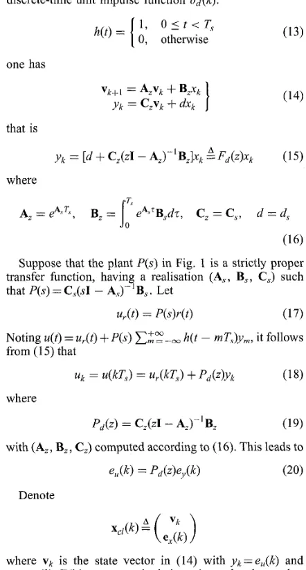
h(t - kT,)xk, where h(t) is the response of the time-invariant zero-order hold H to the discrete-time unit impulse function dd(k):

1, O l t < T , 0, otherwise

h(t) =

one has

that is

A

ylr [d

4-

c,(zI

- A,)--'B,]X/~ zFd(z)xk (15)

where

T,

z , B, =

lo

eA,$'Bsd7, C , = C , , d = d,,

A == &TT

(16)

Suppose that the plant P(s) in Fig. 1 is a strictly proper transfer function, having a realisation (A,, , B,, C , ) such that P(s) = C,&J - A,)-'B,,. Let

u,.(t) = P(s)r(t) (17)

Noting u(t) = u,.(t) +P(s)

CtZ-,

h(t - nzTJy,,, it follows

from (1 5) that

U k = 4 k T J = u,(lcT,)

+

Pd(4Yk (18) where

P ~ ( z ) = C,(ZI - AJ'B, (19)

e l m = M z ) e y ( k ) (20)

with (A,, B,, C,) computed according to (1 6). This leads to

Denote

where vk is the state vector in (14) with yk = e,,(k) and

xk

= e,(k). With some manipulations, it can be shown that

where

Similarly, one has

Remark 1: It is easy to see that A,i is the transition matrix of the digital control system depicted in Fig. 2. This is actually the discrete-time counterpart of the hybrid control system in Fig. 1. It was shown in [18] that the hybrid system is stable if and only if its discrete-time counterpart is stable. Therefore, H J z ) and H,(z) are stable transfer functions.

Since the quantisation errors E,(k) and E,(,%) are statisti- cally independent white sequences (see (9)), it follows that

e,(k) and e,,(k) are wide-sense stationary sequences. Denote

L(0

A

E[e,(k)e,(k -

01

as the autocorrelation function of e,(k) and T,(z) the corresponding spectral density function. According to the well known results in [19], one has

ru(z)

= H , ( ~ ) H ; ( Z - ' ) G ; (25)

and

4

tr [ B z

W$

B,,]

06

(26)

where tr[.] denotes the trace operator and

Wt

is the observability gramian of the realisation of H,(z) (see (24)):

satisfying

Remark 2: The expression given in (26) for the output error variance is based on the digital control system shown in Fig. 2, since the variance is evaluated at the sampling points. This means that the inter-sample behaviour of the output error is not taken into account.

Looking at (7), one can see that the output error of the sampled-data system is the output of the plant excited via a zero-order hold H with an error sequence evaluated with the digital system (23), where the sampling frequency is

f s = 1 / T s . Denote H(s) as the Laplace transform of h(t) defined in (1 3). It turns out that

+03

k = - c c

AU(t> =

c

4l(t - kT&(k) (28)

Fig. 2 system

Block-diagram of the equivalent discrete-time feedback

[image:3.616.51.272.75.486.2] [image:3.616.51.271.86.247.2]

where $(t) is the impulse response of the continuous-time system P(s)H(s). Therefore, the output error variance of the sampled-data system is

(29)

with y,(l) = E[e,(m

+

l)e,(m)] the autocorrelation function

o f

e,(k). Remark 3

0 It is interesting to note that E [ ( A u ( ~ ) ) ~ ] is a periodic

function in t with period T,.

0 y,(Z) can readily be evaluated and, since HJz) is stable,

e,(Z) is a well-behaved sequence.

0 When the plant is unstable, $(t) is an unbounded

sequence [Note 11. This is a serious problem for evaluating

E [ ( A u ( ~ ) ) ~ ] numerically. To overcome this problem we can replace the continuous time plan P(s) with its digital connterpart but with a much higher sampling frequency, denoted as f s = l/ps, than

A.

which is used in digital controller.

L e t z = Nfs with N a large integer. It follows from (15) and (1 6) that

}

(30)

V m y =

A&

+

B,Z,(m)

Au(mT7) = C,v,

where (A,, B,,

c,)

is given by (16) with Tv replaced with

T,

= T,/N and

(31)

A +O0

q m )

=

c

e,,(k)v,(m - k N ) k=-ffi

with qlv(m) the (dismete-time) window function:

Denote 2 as the shift operator, corresponding to sampling frequency

&,

and-

E,@)

the %transform of

Zy(m), we then have E@) =

c:Z-,

i?y(m)Y-" =

[(I - ZN)/(l - 5-')]Ey(2N), where E J z ) is the z-trans- form of e,(k) corresponding to the sampling frequency

fs

.

According to (23),

(33)

with EJz) and E,(z) the z-transforms of E,(k) and ~ , ( k ) , respectively. Therefore, the %transform of Au(mT,J is equal to

where

Pd(Z)

is the discrete-time counterpart of P(s),

obtained from (15) and (16) by substituting T, with

T3

= TJN. This means that

Note 1: Though 4(t) (that is, P(s)H(s)) may be unstable, Au(t) is a stable sequence since the sampled-data system is assumed stable. In fact, there is a pole-zero 'cancellation' between P(s)H(s) and Hy (z).

250

where i5x(m) and Z,(m) are defined in the same way as i?,(m)

in (31). It follows from (9) that

q N ( m - k N )

which is periodic in m with period equal to N.

Theorem 2: Let

w,

be the output of a stable transfer function H$z) = HkzYk excited with a sequence E , .

If E [ E ~ + l ~ m J is a periodic function in m with a period N, so

is E[w,+~w,]. Denote

A 1 N-1 A 1 N - l

Y,(O =

E [ E ~ + ~ E L I ~

Y ~ ( O

=

C

~[w,n+lwLI (37)

m=O m=O

Let r,(z) and r,(z) be their corresponding z-transforms. Then

r,(z) = H(z)17,(z)HT(z-') (38)

Proofi It follows from w, = Hlc~,-k that

+oo +oo

E [ w m + l w ~ l k,=O k2=0 H k l E [ E ( m - k 2 ) + ( l - k l +k2)E&-k2)]Hk:

(39)

Clearly, it is periodic if E[E,,+~E;] is periodic. Based on the above equation, one has

(38) follows by applying z-transformation to both sides of

(40).

0

Denote

It can be shown that

and that its %transform, denoted as

I?,(?),

is

Let

Tu@)

be the %transform of

1

Au((m

+

l)?,)Au(m?;.)

(42)

applying theorem 2 leads to

N m=O m=O

Similarly to (25) and (26), the averaged output error variance of the sampled-data system can be written as

1 N-1

m=O

YJO) = E[{Au(m?,)}2] = tr[W]o; (44)

where

(45)

The averaged roundoff noise gain, denoted as G, is defined as

G=- A ?U(O)

4

and therefore

G = tr[W] (46)

2.2 Realisation dependence

Let (Ac/, Bel, Ccl, De/) and (A:*,

&,

C% be two realisations of HJz) defined by (21) and (22), correspond- ing to the two digital controller realisations

RA(A,

B? C , d )

R,

A

(A,,, B,,

c,,

d )

and

that are related with (3), respectively. It can be shown that

(47)

It then turns out that

H,(Z) = H:(z)

(:

:)

where HE@) is independent of T, and hence

T O T O

w = ( o

J T w o ( 0 1)

where Wo is similar to \iir defined in (45) but corresponds to the controller realisation Ro

.

Let

w q

w

w

Q )

12 w2 1

and

have the same partition as

(E

!)

It is easy to see that W =TTW,T, Q = Q o and hence

G = tr[TTW0T]

+

tr[Q,] (49)

Remark 4: For the equivalent discrete-time feedback system shown in Fig. 2, the averaged roundoff noise gain, denoted was Gd, is defined by GdAE[ei(k)]/oi. It

follows from (26) that Gd = tr[BclWtBcl]. can show that

Gd = tr[TTWiT]

+

tr[Q:] where W i and Q t are independent of T.

Similarly, one

(50)

Clearly, the averaged roundoff noise gain G (or Gd) can be divided into two parts: one is a function of the controller realisation, and the other is a constant, having nothing to do with the controller structure.

3 Dynamic range of states and optimal controller realisations

On the one hand, G is a function of realisation and hence can be made as small as possible with 'small' T. The dynamic range of the states in (l), on the other hand, varies dramatically with realisations. From a practical point of view [Note 21, one wishes that all the states have the same dynamic range. To do so, the actually implemented realisa- tion must be scaled.

The classical Z2-scaling on the states implies that the variance of each state is all equal to one when the input signal r(t) is a white noise with unit variance. Denote K%[xkx:] as the covariance matrix of the state vector of the controller, corresponding to realisation R. The &scaling (see, e.g. [11, 121) implies that the diagonal elements of K satisfy

K(i, i) = 1, V i (51) Let us re-visit (18). According to Theorem 1,

u,(lcT,,) = C,(zI - Az)-'slc, where

T,

s k

I,,

eA.'B,r((k

+

l)T, - z)dz (52)

Therefore, uk = c,(zI - AZ)-'(sk

+

Bzyk), which is equiva-

lent to

( 5 3 )

Combining (53) with (l), one has

This means that

(55)

Since r(t) is a white noise of unit variance, i.e.

E[r(t

+

z)r(t)] = d(z). It follows from the expression (52)

for s k that

that is

(57)

It is easy to see that, in the above equation, the term inside {.} is equal to zero for all k, except

IC=

0 for which it is equal to B:eAT'. We then have

y$(k) E [ S k + m S i ]

=

:

j

eA~'BB,B~eAT'dzG,(k>

5

rod&) (58) which implies that s k is a wide-sense stationary sequence

and so is

It follows that the latter has a power density function given by

Denoting

with I';I2 square root matrix of

r0,

one can see that

where

W,

, called the controllability gramian correspond- ing to (Acl, BJ, satisfies

*,

= A,,W,A;

+

B,B,< (61) Let

where K has the same dimension as that of A. It follows from (47) that

that is

K = T-'K0TdT (64)

where KO is a positive-definite matrix independent of T, corresponding to the controller realisation Ro

.

The above equation means that for a given controller realisation, say Ro, the 12-scaling can be achieved by applying a diagonal transformation T d = diag{ yl,

. . .

,

V k , .

. .

, y,,> with

W k =

Jm,

V k

This transformation leads to an Z2-scaled realisation, denoted as

RF,

that has almost the same structure as Ro and can prevent the controller from overflow. But it is usually not the best one since it may have a very large averaged roundoff noise gain G.

The optimum realisations of the digital controller to the hybrid system depicted in Fig. 1 are the solutions to the following minimisation problem:

min G (65)

R E sc,,

In the next Section, we will discuss how to compute the newly derived measure G and hence to solve for the optimum realisation problem (65).

subject to (51)

252

4 Computing optimal realisations

The l2 dynamic range constraint (51) defines a set of controller realisations, denoted as SF,, in which each realisation satisfies

(66)

Noting the fact that tr[Qo] is independent of T, the optimum controller realisation problem under 12-scaling constraint can be specified as

(T-'KOT-T)(i, i) = 1, for i = 1 , 2 ,

. . .

, n,

min tr

[

T T WoT] T:det(T)#O

subject to (66)

This problem was solved for independently in [ l l , 121. In what follows, we present an alternative approach to solve the optimisation problem (67) and provide an analytical solution.

Lemma 1: Let KO 2 0 be a given n, x n, matrix and T = T l V a non-singular matrix of the same dimension, where V is an orthogonal matrix. There exists a T such that (66) holds if an only if

tr[T;'KoT;T] = n, (68)

€'roo8 The necessary condition is obvious, and we prove the sufficient condition. B a singular value decomposition (SVD), T I ' K o T I T = VOZVO, where

Z

= diag(o1,.

.

. ,

crac> ? 0 and VO is some orthogonal matrix. So, T-lKOT-T=

aTxo

with = VOV Using the numerical algorithm given in [12], one can find a such that

aTZV

has its diagonal elements all equal to one, which means

P

v

=

v;T?

0

min tr [T WoTI

]

(69)

With Lemma 1, (67) can be rewritten as

T, :det(T,)#O n,=tr[T;' KaTFT]

This problem can be solved for using the Lagrange multi- plier method. Noting tr[TrWoT1] = tr[WoP1] and tr[TI'KOTIT] = tr[KoPT1], where

P,LT,TT

we define the Lagrangian

L(P,, A) tr[WOPl]

+

A(tr[K,P;'] - n,) (70)

The optimal P1 should satisfy aL/aPI = 0 and aL/aA, = 0,

which leads to

(71)

I

W0 = AP;'KoPT'

n, = tr[K,P;']

The first equation of (71) implies A > 0 and can be rewritten as

which suggests that 3L'/2Kh'2P;1Kh/2 is a square root matrix of Kh/2WoKA'2. Since the latter is a positive-definite matrix, its square root matrix is unique. Therefore

(73) (KA/2W K'l2 112 = ;11/2KA/2p;lK,!,/2

0 0 )

which leads to

(74) p _{1 -} - A'/2K'/2 K'l2W K1l2 -'/2K'/2 _{o ( 0 0 0 ) 0}

With the second equation of (71), one has

Therefore

(76) As a summary, we then have the following theorem:

Theorem 3: The solutions to (67) are characterised by

Topt = P;l2V (77)

where P I is given by (76) and V is any orthogonal matrix such that the diagonal elements of VTP, 1/2KoP,'/2V are all equal to one; the minimum of the averaged roundoff power gain with l2 scaling is equal to

(5

Ok)'

+

tr[Qol (78)

k= 1

Gmijt =

n,

where {a;} is the eigenvalues set of KoWo.

Prooj First of all, all the solutions to (67) belong to the similarity transformation set defined by (77). It is easy to verify that, with Top, l/given by $77),

This means that Top, defined in (77) is actually the complete solution set of (67). Noting the fact that Kh'2WoKh" and WoKo have the same eigenvalues, (78)

follows.

0

With such a Topt and the given initial realisation Ro, one can obtain an optimal controller realisation of the sampled- data system, denoted as Rupt, using (3).

It is easy to understand that the roundoff noise gain Gd of the digital closed-loop system can be minimised and the corresponding optimal transformations can be obtained in the same way. The optimal controller realisations so obtained are denoted as Rfpt [Note 31. Compared with Rapt, R$ is 'locally' optimal since Gd is a measure that does not take into account the inter-sample behaviour of the sampled-data system.

tr[T$tWOTopt] =tr[P?2W0Pi'2] =(tr[(KO WOKO 1/2 ) I2 I) /nc.

5 Design example

We now present a design example to illustrate the design procedure. The transfer function of the plant is

1 . 6 1 8 8 ~ ~ - 0.157% - 43.9425

P(s) =

s5

+

1 . 1 7 3 6 ~ ~

+

2 8 . 0 7 3 7 ~ ~

+

2 7 . 9 1 8 7 ~ ~

+

0.0186s A stabilising (continuous-time) controller CJs) is designed and the transfer function is

0 . 0 4 6 ~ ~

+

1 .5862s5

+

3 . 0 9 ~ ~

+

4 4 . 3 ~ ~

s6

+

3 . 7 6 6 ~ ~

+

3 4 . 9 5 0 9 ~ ~

+

1 0 6 . 2 ~ ~ +42.7785s2

+

0.02867s

+

1.58 x

CAS) =

+

1 7 9 . 2 ~ ~

+

166.43s

+

0.0033 With

fs

= 1 Hz, we obtained the discretised plant Pd(z)

and controller Cd(z), both are presented with their control-

Note 3: R$ are different from the classical optimal realisations which are obtained by minimising Gd with the constraint &(i, i) = 1, Vi, where Kd is similar to the K matrix but corresponding to the equivalent digital control system.

IEE Proc.-Control Theory Appl., Vol. 149, No. 3, May 2002

lable realisations, denoted as R, and R,, respectively. R, is given by

13.3555 -4.9154 4.0734 -1.8227 0.3093)

0

0

:1

I

0 0 0 1

1 0 0 0

0 1 0 0

0 0 1 0

B, =

i"1

0

C , = (-0.1183 -0.7249 0.6878 -0.6510 -0.0425)

R, is given by

A, =

2.1016 -2.2306 1.4467 -0.4901 0.1954 -0.0231

1 0 0 0 0 0

0 1 0 0 0 0

0 0 1 0 0 0

0 0 0 1 0 0

0 0 0 0 1 0

/ l \

B c = [ J

c,

=

(0.1971 -0.7401 1.1527 -1.0041 0.4857 -0.0912),

d, = 0.0460

We point out that the coefficients of P&) and Cd(z) are presented in FORMAT SHORT (MATLAB) and hence only the first four significant digits in fractional part of each parameter are displayed. In the sequel, the FORMAT SHORT display is assumed. The poles of the ideal closed-loop system and the corresponding absolute values can be computed and they are all inside the unit circle. Clearly, this digital closed-loop system is stable and hence so is the sampled-data system.

With

R,

as the initial digital controller realisation and

N = 11 1 in (45), we compute the corresponding KO, Wo and W;, based on which three 12-scaled controller realisa- tions RZ.", Rfp, and R,, are obtained, where RY is obtained from R, with a diagonal transformation, RZpf and Rapt, as

defined before, are the optimal realisations that minimise

Gd and G, respectively. Table I shows the averaged round- off noise gain of each realisation. The results in Table 1 are self-explanatory. Both the Rtpt and R,, yield a much smaller averaged roundoff noise gain than RF. Comparing

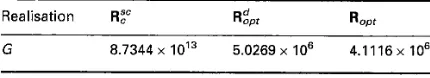
Table 1: Comparison of the averaged roundoff noise gains for the three 12-scaled realisations

Realisation RF RZPt R o p t

G 8.7344 x IOl3 5.0269 x IO6 4.1116 x IO6

[image:7.615.289.504.681.720.2]

the optimum realisation Ropr with R&, one can see that the averaged roundoff noise gain of the former is about 80% of the latter.

Though it is very hard to compute the averaged roundoff noise gain (see (44)-(46)) with simulation data, it is expected that Ropt or Rtpt should have a much smaller output error variance than R;,‘. Also R,, should have a smaller output error variance than Rtpt. To confirm these, some simulations have been conducted. In Fig. 1, the input signal r(t) is replaced with a white sequence of 100 000 points, generated with unit variance using the command

randn in MATLAB. The continuous-time plant is replaced with its discrete-time counterpart obtained using fast sampling

(h

= 10h. = 10 Hz). The digital controller is implemented with (4), where the quantiser Q [ p ] rounds the fractional part of signal p into 16 bits. The variance of the error sequence between the ideal output and the actual one of the sampled-data system for each of the three controller realisations is computed with the same input se uence. For RS,C, the variance is 3.2708 x lo6, while for [image:8.613.345.554.48.240.2]

R,,,.

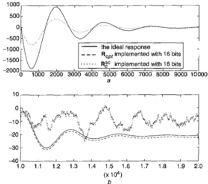
and Rapt, we have 8.1846 and 6.23 18, respectively. Fig. 3 shows the unit-step responses of the sampled-data system, where the solid line is for the ideal response, while the dashed and the dotted lines are for 16-bit implemented Ropt and RF, respectively. Clearly, the response corre- sponding to RF is far away from the desired one, while the one corresponding to Rapt is very close to the ideal response. Fig. 4 compares the ideal unit-step response of the sampled-data system with those of 16-bit implemented Rapt and Rfpt, respectively. It can just be seen visually that the output error for R$,t is larger than that for Rapt.

B

6 Conclusions

We have addressed the optimum digital controller structure problem in a hybrid system with roundoff noise considera- tion. Our contribution has been threefold. The first one is to have given a thorough analysis of the effect of roundoff noise in the digital controller on the output of the system. Based on this analysis, a new measure has been proposed. This measure, unlike the existing ones, is derived for the

the ideal response

- - -

Ropr implemented with 16 bits

RgC implemented with 16 bits

-1 500 -2000

0 1000 2000 3000 4000 5000 6000 7000 8000 9000 10000

a

10 r I I I r I i I I

-40

1.0 1.1 1.2 1.3 1.4 1.5 1.6 1.7 1.8 1.9 2.0 b

( X io4)

Fig. 3 Unit-step responses of the sampled-data system (x-axis in second)

Note that in the first 10000 seconds (a), with the given y-axis range, the differences for the ideal response and that of R,,,, implemented with 16 bits cannot visually be seen

254

-1 000 -1 500 -2000

[image:8.613.107.319.479.667.2]

0 1000 2000 3000 4000 5000 6000 7000 8000 900010000

...

-1 5

-20

-30 -35

1 0 1 1 1.2 1 3 1.4 1.5 1.6 1.7 1.8 1.9 2 0 ( ~ 1 0 ~ )

b

Fig. 4 Unit-step responses ofthe sampled-data system (x-axis in

second)

Note that in the first 10000 seconds (a), with the given y-axis range, the differences for the three responses cannot visually be seen

hybrid system rather than its discrete-time counterpart and hence can take the inter-sample behaviour into account. The second contribution is to have given a method to evaluate this measure by fast sampling plant, which can avoid the numerical problem involved in computing directly the newly defined measure. The exact expression for the covariance matrix of controller state vector has also been derived in order to scale the realisations with 12 norm.

It is shown that the proposed new measure is controller realisation dependent, and the third contribution of this paper is to have presented an analytical solution to the optimum controller structure problem. A design example has been given to illustrate the design procedure and to confirm the theoretical results.

7 Acknowledgments

J. Wu and S. Chen are grateful for the support of the UK Royal Society under a KC Wong fellowship

(RL/ART/CN/XFI/KCW/11949).

References

LI, G., and GEVERS, M.: ‘Optimal finite precision implementation of a state-estimate feedback controller’, IEEE Trans. Circuits Syst., 1990,38, (12), pp. 1487-1499

GEVERS, M., and LI, G.: ‘Parametrisations in control, estimation and filtering problems: accuracy aspects’ (Springer Verlag, London, Communication and Control Engineering Series, 1993)

MADIEVSKI, A.G., ANDERSON, B.D.O., and GEVERS, M.: ‘Opti- mum realizations of sampled-data controllers for FWL sensitivity mini- mization’, Automatica, 1995, 31, (3), pp. 367-379

FIALHO, I.J., and GEORGIOU, T.T.: ‘On stability and performance of sampled-data systems subject to wordlength constraint’, IEEE Trans. Autom. Control, 1994, 39, pp. 2476-2481

FIALHO, I.J., and GEORGIOU, T.T.: ‘Optimal finite wordlength digital controller realizations’. Proc. American Control Conf., San Diego, USA, 2 4 June 1999, pp. 4 3 2 6 4 3 2 7

LI, G.: ‘On the structure of digital controllers with finite word length consideration’, IEEE Trans. Autom. Control, 1998, 43, ( S ) , pp. 689-693 ISTEPANIAN, R.H., L1, G., WU, J., and CHU, J.: ‘Analysis ofsensitivity measures of finite-precision digital controller structures with closed-loop stability bounds’, IEE Proc., Control Theory Appl., 1998, 145, ( S ) , pp. 4 7 2 4 7 8

CHEN, S., WU, J., ISTEPANIAN, R.H., and CHU, J.: ‘Optimizing stability bounds of finite-precision PID controller structures’, IEEE Trans. Autom. Control, 1999,44, (1 l), pp. 2149-2153

9 WU, J., CHEN, S., LI, G., and CHU, J.: ‘Optimal finite-precision state- estimate feedback controller realizations of discrete-time systems’, IEEE Trans. Autom. Control, 2000, 45, (8), pp. 1550-1554

10 CHEN, S., ISTEPANIAN, R.H., WU, J., and CHU, J.: ‘Comparative study on optimizing closed-loop stability bounds of finite-precision controller structures with shift and delta operators’, Syst. Control Lett.,

2000,40, (3), pp. 153-163

11 MULLIS, C.T., and ROBERTS, R.A.: ‘Synthesis of minimum ronndoff noise fixed-point digital filters’, IEEE Trans. Circuits Syst., 1976, 23,

12 HWANG, S.Y.: ‘Minimum nncorrelated unit noise in state-space digital filtering’, IEEE Trans. Acoust., Speech Signal Process., 1977, 25, (4), pp. 273-28 1

13 ROBERTS, R.A., and MULLIS, C.T.: ‘Digital signal processing’ (Addison Wesley, 1987)

14 AMI, G., and SHAKED, U.: ‘Small roundoff realization of fixed-point digital filters and controllers’, IEEE Trans. Acoust., Speech Signal Process., 1988, 36, (6), pp. 880-891

pp. 55 1-562

15 MORONEY, P., WILLSKY, A.S., and HOUPT, P.K.: ‘The digital implementation of control compensators: the coefficient wordlength issue’, IEEE Trans. Autom. Control, 1980, 25, (4), pp. 621-630 16 WILLIAMSON, D., and KADIMAN, K.: ‘Optimal finite wordlength

linear quadratic regulation’, IEEE Trans. Autom. Control, 1989,34, (12),

17 LIU, K., SKELTON, R., and GRIGORIADIS, K.: ‘Optimal controllers for finite wordlength implementation’, IEEE Trans. Autom. Control,

18 CHEN, T., and FRANCIS, B.A.: ‘Input-output stability of sampled data

I9 ZSTROM, K.J.: ‘Introduction to stochastic control theory’ (Academic pp. 1218-1228

1992,37, pp. 1294-1304

s stems’, IEEE Trans. Autom. Control, 1991, 36, (I), pp. 50-58 Press, New York, 1970)