Volume 4, No. 4
December 1999
Exchanges
Exchanges No. 14
News from the ICPO
2
A Common Mode of Subseasonal and Interannual Variability
4
of Indian Summer Monsoon
Interannual to Decadal Variability of the Atmospheric Circulation in Coupled
7
and SST-forced GCM Experiments
A Perspective on the Ocean Component of Climate Models
11
Coupled Climate Modelling at GFDL: Recent Accomplishments and Future Plans
15
Climate Variability at Decadal and Interdecadal Time Scales
21
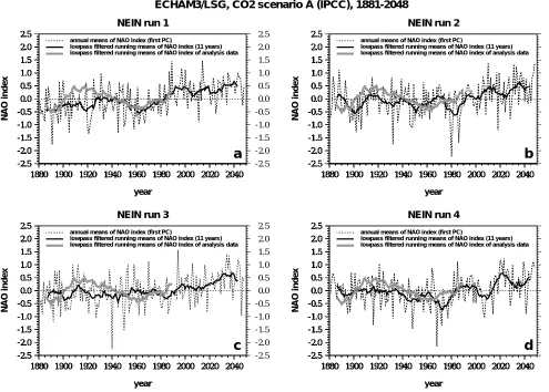
Climate change signals in the North Atlantic Oscillation
25
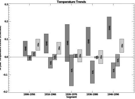
Natural and Anthropogenic Causes of Twentieth-Century Temperature Change
29
U.S. CLIVAR Defines Objectives and Approach
33
4th International Conference on Modelling of Global Climate Change
35
and Variability
Third session of the JSC/CLIVAR Working Group On Coupled Modelling
37
Second International WCRP Conference on Reanalyses
38
News from the ICPO
Dr. John Gould, Director, International CLIVAR Project Office,
Southampton Oceanography Centre, Empress Dock, Southampton, SO14 3ZH, UK
corresponding e-mail: [email protected]
This issue of Exchanges
This latest issue of Exchanges contains some in-teresting papers on a variety of topics largely relating to the role of modelling activities in CLIVAR. As you may know, CLIVAR oversees its modelling development through two panels, one the WCRP Working Group on Coupled Modelling that is chaired by Lennart Bengtsson and the second the CLIVAR Working Group on Seasonal to Interannual Prediction chaired by Steve Zebiak. As their names imply these panels deal respectively with the long and short timescale climate processes of interest to CLIVAR (monsoons and ENSO events through to an-thropogenic change). Both WGs have met recently. A report of the WGCM is included on page 37 and a report of the WGSIP will be given in the next issue.
Given the sparse nature of the observational cli-mate data base, modelling activities are the key to better understanding the climate system and its variability. It seems likely that the requirements of climate modelling will stretch the limits of available computer capability for the foreseeable future as models move to higher reso-lution in both atmosphere and ocean and as long ensem-ble runs are required.
Second Conference on Reanalyses and 4th International Conference on Global Climate Change and Variability
This issue of Exchanges, highlighting some recent activities and findings in the field of climate modelling has also been motivated by two major meetings in late summer and fall: The Second Conference on Reanalyses held in late August in Reading, UK (please find a sum-mary on page 38) and the 4th International Conference on Global Climate Change and Variability that took place in September at the Max-Planck-Institute for Meteorol-ogy in Hamburg, Germany. A report of this meeting is given on page 35. The papers selected for this issue pro-vide an overview about the climate modelling efforts presented on that conference which themes and goals matched perfectly with the CLIVAR requirements in this field of climate research.
First International Conference on the Ocean Observ-ing System for Climate (OceanObs’99)
You will remember that the last newsletter - a bumper edition - was focused on and published to coin-cide with the First International Conference on the Ocean Observing System for Climate in St. Raphael France. It has become known in short by most people as OceanObs’99. I, and many other CLIVAR scientists were among the approx. 350 attendees at this important meet-ing. Its objectives were to identify the appropriate mix of sustained global observations that would be required to address the needs of GOOS/GCOS and of CLIVAR.
A formal report of the Conference is not yet avail-able so what follows is my own personal view. The meet-ing was wide-rangmeet-ing and covered in detail aspects as diverse as satellite remote sensing of the ocean surface, full depth hydrography and tracer measurements, urements from ships of opportunity and acoustic meas-urements of the ocean through invited papers prepared by, in many cases, large groups of co-authors. There were panel discussions that exposed a number of issues and that went on until quite late in the evenings and some excellent posters. It was hard work and was very worth-while but in some senses the real task is still to be done – to distill an appropriate observational strategy that will exploit the strengths of each technique and that can be assembled into a sustainable observing system that will serve both research and operational activities. Details on the conference can be obtained at the conference homepage: http://WWW.BoM.GOV.AU/OceanObs99 which includes all of the contributed papers and a draft of the conference statement. The homepage also con-tains a continuing dialog on the conference papers and conclusions, which encourages community participation through a comment board.
CLIVAR Data Task Team
hours in the sun was well worthwhile and the DTT started to formulate its view of how CLIVAR data should best be managed and made available (together with derived products) to CLIVAR researchers. CLIVAR is probably able to influence the manner in which ocean observa-tions are dealt with in delayed-mode largely through the systems that have served so well in the World Ocean Cir-culation Experiment (WOCE). To this end the DTT en-dorsed many elements of the WOCE data system as be-ing appropriate to fulfil some of CLIVAR’s requirements. These endorsements should help to ensure the continuity of these systems. Of greater complexity are the opera-tional (real-time) systems for both atmospheric and ocean data. Assessing the adequacy of these systems for meet-ing CLIVAR’s needs will be major task for the DTT.
CLIVAR Panels and WGs
The OceanObs meeting was co-sponsored by the CLIVAR Upper Ocean Panel whose chairman Chet Koblinsky, (together with Neville Smith) are to be con-gratulated on their hard work in making OceanObs suc-ceed. The Conference highlighted the broadened role that the CLIVAR UOP should now take (global and not solely confined to upper ocean matters) in light of the close re-lationship between CLIVAR and GOOS/GCOS and of the establishment by CLIVAR of sector implementation panels. Discussion is now taking place to produce re-vised terms of reference for UOP.
The final revisions are being made to the report of the CLIVAR African Climate Study Group. We plan that it should be available early in the New Year. This report will act as the basis for the formulation of a more con-crete plan by the CLIVAR Africa Task Team (CATT) under its chairman Chris Thorncroft of the University of Reading, UK.
Other Meetings
In November the PAGES and CLIVAR again joined forces to hold a workshop on extending the in-strumental record and making it useful for CLIVAR pur-poses in Venice, Italy. The workshop documented im-pressive progress on paleo data analysis, modelling and synthesis. Outstanding results include the synthesis of detailed reconstructions with annual resolution of the past climate over the last 1,000 years that have been pub-lished recently, and which are changing our views on the Little Ice Age and whether their even was a Medi-eval warm period (other than regionally). They provide an extremely valuable basis for advances in our under-standing in natural climate variability and in the climate forcings. Fruitful exchanges between the two commu-nities occurred and a joint research activity for the next
5 years or so has been refined. The next issue of Ex-changes will be a joint one with PAGES and highlight in more detail the accomplishments of this workshop.
I am about to attend the workshop and meeting of the CLIVAR Australian-Asian Monsoon Panel in Hawaii in early December. It promises to be a lively meeting. A number of recent research papers highlight aspects of the role of the Indian Ocean in both the monsoon and in ENSO and I am looking forward to hearing more of this and of hearing how the panel plans to develop a strategy within CLIVAR to better understand the workings of the A-A Monsoon.
National programmes and information flow
It is now a year since the International CLIVAR Conference in Paris. The report has been widely circu-lated and contains the text of the plenary lectures and summaries of the national reports made to the confer-ence It is essential that the CLIVAR SSG and the ICPO are kept well informed about the progress of national programmes for CLIVAR research and in light of this I will be contacting national co-ordinators for CLIVAR requesting updated statements on national plans. Infor-mation flow is a two way process and we are about to make available on the WWW a searchable information source that will enable anyone to find who is doing CLIVAR research on a particular Principal Research Area, in a geographical area or by an individual country. It will we hope include a searchable bibliography of CLIVAR-related papers and reports. The system has been devel-oped by Christine Haas who has been working in Ge-neva on CLIVAR matters for the past year and I think it will prove to be an invaluable asset to CLIVAR. The value will be greatly enhanced as more information is added and kept up to date. That is where all of you CLIVAR researchers can help by feeding new information to the ICPO for inclusion.
Thank you and Happy New Year
Finally I and the SSG co-chairs Kevin Trenberth and Jürgen Willebrand want to thank all of the members of the CLIVAR Panels and WGs who have given their time and energy to the project over the past year. Your contributions are very much appreciated. I would also like to thank the ICPO staff who have supported meet-ings, prepared reports and particularly Andreas Villwock who has worked to ensure that CLIVAR Exchanges has appeared at the appointed times and has increasingly fo-cused in science issues.
And of course the co-chairs and all of the ICPO staff send you best wishes for Christmas and for the year 2000.
1. Introduction
Summer monsoon rainfall is the life-blood of the agrarian societies of subtropical Asia. Dynamical sea-sonal forecasting of the Asian summer monsoon (ASM), if successful, would revolutionize the ability of govern-ments of agrarian societies dependent on monsoon rain-fall to deal with the prospective impacts of a weak or strong monsoon. Using ensembles of simulations with numerical weather prediction models, dynamical sea-sonal predictions have the potential to provide probabilistic forecasts. Based on the dispersion of the ensemble members it would be possible to establish con-fidence thresholds on the forecast, and to gain some in-sight on the potential regionality of the rainfall anoma-lies. However, to date, dynamical seasonal predictabil-ity of the boreal summer monsoon system has been prob-lematic (Brankovic and Palmer, 1999), possibly due to model errors in the mean monsoon simulation which are still substantial enough that the signal being sought is smaller than the systematic bias. It has also possible that limited predictability of the monsoon may arise due to chaotic variability on subseasonal time-scales. However, it has been hypothesized that the slowly varying com-ponents of the climate system, such as sea-surface tem-perature and/or land-surface interactions, may predis-pose chaotic modes of subseasonal variability (or weather) into preferred states resulting in an increased probability of a wet or dry monsoon depending upon the sign of the forcing (Palmer, 1994). Evidence for these types of perturbations has been manifest in simulations with models of varying complexity (Palmer, 1994; Fennessy and Shukla, 1994; Ferranti et al., 1997; and Webster et al., 1998). In this paper we test this hypoth-esis using the NCEP/NCAR reanalysis (Kalnay et al., 1996) for June-September 1958-97. Sperber et al. (1999) present a more in-depth analysis of the dominant modes of ASM variability.
2. Interannual and Subseasonal Variability
Using daily rainfall and 850hPa winds from the reanalysis for June-September 1958-97 we have inves-tigated the link between subseasonal and interannual variability of the Asian summer monsoon (Sperber et al., 1999). The 850hPa winds are an excellent candidate for analysis since they encapsulate both the large-scale and regional-scale structures of the monsoon circulation. Here we concentrate on the modes that are most impor-tant for Indian monsoon. We have used empirical orthogonal function (EOF) analysis to identify the domi-nant spatio-temporal modes of variability on (1) interannual time-scales using seasonal anomalies, and (2) subseasonal time-scales using daily anomalies (climatological daily means removed).
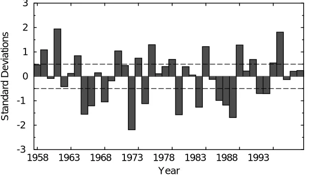
The most accurate estimate of rainfall available during the summer monsoon is that over India, collected through an extensive gauge network (Parthasarathy et al., 1994). Figure 1 shows the interannual variations of all-India rainfall. Associated with the interannual varia-tion of all-India rainfall is a characteristic pattern of 850hPa wind anomalies (Fig. 2a, see page 19), comprised of cyclonic anomalies over the bulk of the Indian sub-continent, with anticyclonic anomalies located further south, and to the north in the foothills of the Himalayas. The wind pattern has been constructed from the differ-ence of the composites based on years of above-normal versus below-normal all-India rainfall using the +/-0.5 standard deviations thresholds given in Fig. 1. The com-posite difference is nearly identical to the comcom-posite for 1979-95 (Annamalai et al., 1999), when the reanalysis is believed to be more reliable due to the incorporation of satellite data in the assimilation, thus indicating the robustness of this pattern of anomalies throughout the 40-year reanalysis. Similarly, relative to the observed all-India rainfall, Fig. 2b shows the regional distribu-tion of rainfall anomalies from the reanalysis. The en-hanced rainfall over India is consistent with the pres-ence of cyclonic anomalies over the subcontinent, while the below normal rainfall to the south and west of India corresponds to the anticyclonic anomalies. This
A Common Mode of Subseasonal and Interannual Variability
of Indian Summer Monsoon
Kenneth R. Sperber1
, Julia M. Slingo2
, and H. Annamalai2
1PCMDI, Lawrence Livermore National Laboratory, P.O. Box 808, L-264
Livermore, CA 94550, USA
2Centre for Global Atmospheric Modelling, Dept. of Meteorology, University of Reading, Earley Gate,
P.O. Box 243, Reading RG6 6BB, UK
interannual signal in the reanalysis precipitation (Fig. 2b) has been confirmed since this pattern agrees well with that obtained for the period 1979-95 (Annamalai et al., 1999) from compositing observed rainfall estimates constructed from satellite and surface gauge data (Xie and Arkin, 1996).
EOF analysis of the seasonal anomalies has suc-cessfully identified a mode which has a very similar pat-tern to that obtained by compositing on all-India rain-fall, particularly in the vicinity of India (Fig. 2c). The anticyclonic/cyclonic/anticyclonic pattern is clearly seen in EOF-4. Similarly, the composite rainfall anomalies calculated relative to the principal component (PC) time series of EOF-4 (Fig. 2d) correspond closely to that cal-culated relative to observed all-India rainfall (Fig. 2b), particularly over India, and much of the Asian summer monsoon region. Importantly, the PC time series of EOF-4 has a correlation of 0.60 (significant at >1% level) with respect to the observed seasonal mean all-India rain-fall. Thus, the similarity of the spatial pattern of EOF-4 and its associated rainfall anomalies (Figs. 2c, d) with that of the composites based on all-India rainfall (Figs. 2a, b), plus the high temporal correlation of the PC time series of EOF-4 with observed all-India rainfall provides confirmatory evidence that the EOF analysis has ex-tracted a physically realistic mode of Indian summer monsoon variability.
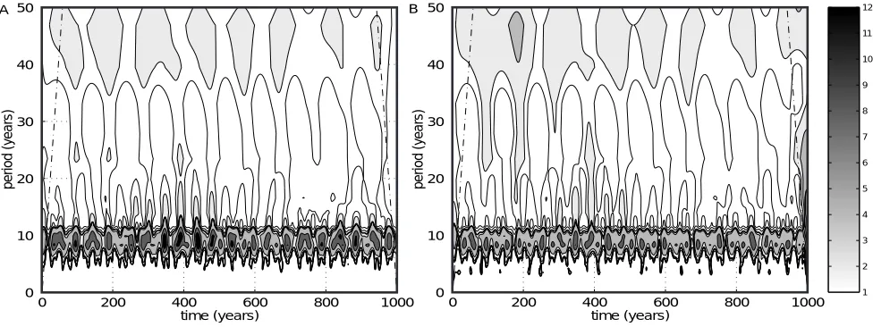
A main tenet of the hypothesis that perturbations to subseasonal variability control the interannual vari-ability is that the patterns of subseasonal and interannual variability should correspond (Palmer, 1994). We have found that the third mode of subseasonal variability (EOF-3; Fig. 3a, see page 19), extracted from an analy-sis using daily 850hPa wind anomalies, exhibits the anti-cyclonic/cyclonic/anticyclonic pattern in the vicinity of India obtained using the interannual anomalies (Figs. 2a, c). Time series analysis of the PC time series indicates this mode of variability to be dominated by time-scales of 7-40 days, the time-scales that are considered impor-tant for active/break cycles of the monsoon. This mode
captures the main elements of the well documented pat-tern associated with active (wet) versus break (dry) phases of the Indian summer monsoon (Ramamurthy, 1969; Lau and Chan, 1986; Webster et al., 1998).
The composite difference of daily rainfall from the reanalysis (Fig. 3b), based on +/-1 standard devia-tion thresholds of the PC time series, exhibits a nearly identical pattern of rainfall anomalies as found on interannual time-scales (Fig. 2b, d). These results sug-gest the viability of the link between subseasonal and interannual variability. Closure of the link between the subseasonal and the interannual variability of Indian summer monsoon is established by demonstrating that the subseasonal mode projects on to the interannual vari-ability. The link is established by demonstrating the im-portance of the subseasonal mode for high frequency variations of all-India rainfall. This is shown in Fig. 3c, in which the PC time series of the subseasonal mode and the variations of observed daily all-India rainfall (both subject to a 5-day running mean) are plotted for 1987. The variations of the all-India rainfall correspond closely to the changes of the PC time series, particularly during the months of June and July. The correlation of these two time series is 0.59, significant at >5% level (assuming 10 degrees of freedom or greater during the 122 day season). This level of correlation is typical of the years during which the daily all-India rainfall data are available (1971-95). Thus, this mode of variability is an important modulator of the short-term variations of Indian summer monsoon rainfall.
It should be noted that 1987 was a year of below-normal all-India rainfall, and this is clearly reflected in the bias of the PC time series and the daily all-India rain-fall departures towards negative values during this sum-mer (Fig. 3c). The seasonal average of the daily PC time series is an integrated measure of the influence of the subseasonal mode on the total seasonal anomaly. Calcu-lating the seasonal average of PC-3 for each summer 1958-97, and correlating with observed all-India rain-fall (Fig. 1) results in a coefficient of correlation of 0.67
1958 1963 1968 1973 1978 1983 1988 1993
Year -3
-2 -1 0 1 2 3
[image:5.595.58.371.75.251.2]Standard Deviations
(significant at >1% level), thus directly linking the interannual variations of observed all-India rainfall to variations of the subseasonal mode. The seasonal aver-ages of PC-1, PC-2, and PC-4 have much weaker corlations with all-India rainfall (0.23, -0.13, and 0.04 re-spectively) indicating that the projection of these subseasonal modes on to interannual variations of In-dian monsoon rainfall is tenuous at best. Furthermore, as suggested by the negative values of the PC during 1987, the probability distribution function (PDF; Fig. 3d) of the daily PC time series is systematically per-turbed towards negative values during years of below normal all-India rainfall, whereas it is perturbed towards positive values during years of above normal all-India rainfall. These changes in the means of the PDF’s are significant at >2.5% level.
3. Conclusions and Discussion
We have isolated a mode of variability that projects strongly on to both subseasonal and interannual time-scales of Indian summer monsoon, with this mode ex-erting the dominant influence in the subseasonal and interannual variations of rainfall and lower tropospheric flow over this region. This supports the hypothesis that perturbations to otherwise chaotic phenomena can re-sult in discernible influences on interannual time-scales, even though the impact does not occur to the leading (first mode, Sperber et al., 1999) and the perturbation is not manifested as bimodality, as had been suggested (Palmer, 1994). As yet, the mechanism(s) and boundary forcing(s) that cause the systematic changes in the be-haviour of this linked mode of subseasonal and interannual variability have yet to be determined, but will undoubtedly have a major impact on our ability to predict all-India rainfall. If numerical weather predic-tion models are not able to simulate this subseasonal mode of variability, and the other dominant modes of variability that are important for the Asian summer monsoon in general (Sperber et al., 1999), this would suggest that the present limitations on seasonal predict-ability of ASM may imposed by our limited understand-ing of the complex processes that govern the ocean-at-mosphere-land system rather than by nature itself. To this end, we are currently investigating the models con-tributed to the Seasonal Prediction Model Intercomparison Project (SMIP) initiated by the CLIVAR Working Group on Seasonal to Interannual Prediction (WGSIP). These integrations consist of ensembles of seasonal hindcasts, and the ability of the models to simu-late the hierarchy of ASM modes and their interactions will be investigated to assess the state-of-the-art in sea-sonal forecasting.
Acknowledgments
This work was performed under the auspices of the U.S. Department of Energy Environmental Sciences Division at the Lawrence Livermore National Labora-tory under Contract W-7405-ENG-48. NCEP/NCAR Reanalysis data provided through the NOAA Climate Diagnostics Center (http://www.cdc.noaa.gov/).
References
Annamalai, H., J.M. Slingo, K.R. Sperber and K. Hodges, 1999: The mean evolution and variability of the Asian summer monsoon: comparison of ECMWF and NCEP/ NCAR reanalyses. Mon. Wea. Rev., 127, 1157-1186.
Brankovic, C. and T.N. Palmer, 1999: Seasonal skill and predictability of ECMWF PROVOST ensembles. Quart
J. Roy. Meteor. Soc., submitted.
Fennessy, M.J. and J. Shukla, 1994: GCM simulations of active and break monsoon periods. Proceedings of the International Conference on Monsoon Variability and Prediction, World Meteorological Organization/TD-NO. 619, WCRP-84, Vol. 2, 576-585.
Ferranti, L., J.M. Slingo, T.N. Palmer and B.J. Hoskins, 1997: Relations between interannual and intraseasonal monsoon variability as diagnosed from AMIP integra-tions. Quart J. Roy. Meteor. Soc., 123, 1323-1357.
Kalnay, E., M. Kanamitsu, R. Kistler, W. Collins, D. Deaven, L. Gandin, M. Iredell, S. Saha, G. White, J. Woollen, Y. Zhu, M. Chelliah, W. Ebisuzaki, W. Higgins, J. Janowiak, K.C. Mo, C. Ropelewski, J. Wang, A. Leetma, R. Reynolds, R. Jenne and D. Joseph, 1996: The NCEP/NCAR 40-year reanalysis project. Bull. Amer.
Meteor. Soc., 77, 437-471.
Lau, K.-M. and P.H. Chan, 1986: Aspects of the 40-50 day oscillation during northern summer as inferred from outgoing longwave radiation. Mon. Wea. Rev., 114, 1354-1367.
Palmer, T.N., 1994: Chaos and predictability in forecast-ing the monsoons. Proc. Indian Nat. Sci. Acad., Part A
60, 57-66.
Parthasarathy, B., A.A. Munot and D.R. Kothawale, 1994: All-India monthly and seasonal rainfall series: 1871-1993.
Theoretical and Applied Climatology, 49, 217-224.
1. Introduction
Little is known about the role of the coupling mechanisms between atmosphere and ocean on the interannual to decadal time scales. Numerous experi-ments were investigated using atmosphere GCM with various lower boundary conditions reaching from climatological SST, prescribed observed SST variabil-ity, a mixed layer ocean, and various combinations to a fully interactive ocean (Bladé et al., 1999; Christoph et al., 1998; Davies, 1997; Lau et al., 1996; Moron et al., 1998; Saravanan, 1998). An investigation of the cou-pling mechanisms with coupled and forced GCM ex-periments has been performed by Selten et al. (1999). They systematically investigated the role of coupling in an atmosphere-ocean GCM by performing auxiliary ex-periments with the atmosphere-only and ocean-only GCM, taking fluxes and SST from the coupled simula-tion as boundary condisimula-tions.
The extratropical atmosphere shows widely un-changed patterns of variability, which are not depend-ing on the lower boundary configuration (Saravanan, 1998). Merely slight changes were observed by Bladé et al. (1999). The order of variance of the single patterns and the probability function may be changed (Molteni et al., 1993). Selten et al. (1999) and Christoph et al. (1998) observed the development of spectral peaks in the amplitude spectrum of the dominant modes of vari-ability in the coupled simulation which were absent in the SST forced simulations. Neelin et al. (1999) ascer-tain dominant spectral peaks within their ocean model coupled to stochastically varying atmospheric heat and momentum fluxes. The coupling was implemented by changing the mean and variance of the white noise at-mospheric fluxes depending on SST.
Various conceptional models were build to ana-lyse the role of coupling within the framework of stochastic models (Hasselmann, 1976). Barsugli and
Battisti (1998) investigated a simple stochastically forced energy balance model of the atmosphere ocean system. Their model exhibits an amplification of variance in the coupled in contrast to the uncoupled system. Saravanan and Williams (1998) developed an one-dimensional stochastic model, where the atmosphere was resolved by stochastically varying coherent patterns and was cou-pled to an advective ocean. Their system exhibits spec-tral peaks in the variance spectrum. They conclude that the interaction between a stochastically varying atmos-phere and an advective ocean plays a major role in the development of decal variability.
Our analysis will concentrate on the variability of various variables in different regions in coupled and SST forced GCM experiments. Chapter 2 describes the model simulations and the statistical analysis tools to analyse and compare the variance. The results are presented in chapter 3 for the euro-atlantic (chapter 3.1) and tropical (chapter 3.2) atmospheric circulation.
2. Simulations and Statistics
The analysis is based on an 800-year integration with the Hamburg ECHAM3-T21/LSG (Voss et al., 1998; Roeckner et al., 1992; Maier-Reimer et al., 1993), a coupled atmosphere ocean sea-ice GCM. A time slice of a 100-year period of integration was selected. The monthly mean SST and sea ice boundaries of the time slice coupled simulation were used to perform an en-semble of forced atmosphere-only simulations with the ECHAM3-T21. The ensemble consists of the coupled 100-year integration and four SST-forced simulations differing only in their independent initial conditions. An ensemble mean was calculated summing up the four SST-forced simulations for each time step.
The LSG ocean model is characterised by a largely underestimated tropical SST variability due to the coarse Sperber, K.R., J M. Slingo and H. Annamalai 1999:
Pre-dictability and the relationship between subseasonal and interannual variability during the Asian summer monsoon. PCMDI Report No. 53, http://www-pcmdi.llnl.gov/pcmdi/pubs/ab53.html, Quart. J. Roy.
Meteor. Soc., submitted.
Webster, P.J., V.O. Magaña, T.N. Palmer, J. Shukla, R.A. Tomas, M. Yanai and T. Yasunari, 1998: Monsoons: proc-esses, predictability and the prospects for prediction. J.
Geophys. Res. 103, 14,451-14,510.
Xie, P. and P. Arkin, 1996: Analyses of global monthly precipitation using gauge observations, satellite estimates and numerical model predictions. J. Climate, 9, 840-858.
Interannual to Decadal Variability of the Atmospheric Circulation in Coupled and
SST-forced GCM Experiments
Petra Friederichs and Andreas Hense
Meteorologisches Institut, Universität Bonn, Auf dem Hügel 20, D-53121 Bonn, Germany
resolution of 4° x 4°, whereas the variance amplitude of the extratropical SST variability resembles observational variance.
The Northern Hemispheric winter seasonal means of the investigated atmospheric variables were pooled to one 500-year simulation by lining up the four forced simulations and the one coupled simulation. A principal component analysis was carried out for the pooled simu-lation, obtaining one set of empirical orthogonal func-tions (EOF) for each variable. A Blackman-Tukey spec-trum using Bartlett smoothing was calculated for the principal components (PC) for each simulation (coupled and forced) and the ensemble mean of the forced simulations. The bandwidth and a 95% confidence in-terval for a stochastic process are indicated by two crossed lines. A univariate analysis of variance (ANOVA) was carried out to estimate the SST forced fraction of the total variance in the forced ensemble.
3. Results
3.1 Extratropics
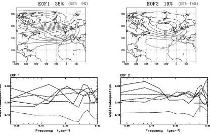
Figure 1 (top) shows the first and second EOF of the euro-atlantic 500 hPa geopotential height anoma-lies. The EOF differ only slightly between the single simulations and there is no significant difference be-tween the patterns of the coupled and the forced simulations. The first EOF shows a NAO-like variabil-ity with the synchronously varying pressure systems over Greenland and westward of Europe. In comparison with observations the dipole pattern is located to far to the north. The fraction of variance linearly explained by the prescribed SST in the PC of the first EOF amounts to 9% of the total variance. The second EOF shows simi-lar structures located further to the south. The SST ex-plained variance fraction is slightly higher with 16% of the total variance.
The variance spectra of the PC (Figure 1, bottom) of the various simulations show a wide spread at all time scales. The spectral variance of the first principal com-ponent of the coupled simulation lies within the range spanned by the spectra of the forced simulations. The ration between the spectral variance of the single forced simulations and the ensemble mean represents an esti-mate of the SST induced fraction of variability. The en-semble mean run shows significantly less variance on all time scales. This reflects the small fraction of SST induced variance already shown with the ANOVA of the PC.
The PC of the second EOF in the coupled simula-tion shows a significant spectral peak at the frequency at about 0.08/a (period of 12 years). It represents a cou-pled mode of variation in the coucou-pled simulation. Here atmospheric anomalies primarily force anomalous SST
through heat and momentum fluxes. The spectral peak is indeed more present in the SST than in the atmos-phere. In the forced simulations the spectral peak van-ishes and the variance spectra of the second PC are white. Thus there is evidence that the coupling between the two climate systems enables the development of coupled variability on preferred decadal time scales. To deter-mine whether the coupled mode resides in the ocean or whether it needs the coupled system to develop has to be examined with auxiliary ocean only simulations. Seltan et al. (1999) did not reproduce the spectral peak in the uncoupled simulations.
3.2 Tropics
Substantial differences result from the analysis of tropical atmospheric variability. Figure 2 shows the first EOF of the zonal eddy streamfunction and the velocity potential at 200 hPa, respectively. The patterns resemble typical anomalies induced by anomalous tropical heat-ing. They can be reproduced with a linear reduced grav-ity model after Matsuno (1966) and Gill (1980).
Although the variability of the tropical SST is largely underestimated by the coupled model the tropi-cal atmospheric circulation of the forced simulations shows substantial SST forced variability. The fraction of SST induced variability amounts to 40% of the total vari-ance of the 200 hPa streamfunction and velocity poten-tial. The PC show significant differences between the forced and the coupled simulations. The coupled simu-lation has a much smaller variance that even falls below the variance of the ensemble mean simulation. Due to the large fraction of SST induced variability the ratio between the variance of the ensemble mean and the forced simulations is larger than for the euro-atlantic geopotential height.
Fig. 1: First and second EOF of the euro-atlantic 500 hPa geopotential height (contour interval: 10 gpm) and spectral analysis of the principal components using a Bartlett spectrum with 22.5 degrees of freedom and a window of 12 years. The solid line represents the coupled simulation, the dashed lines the forced simulations and the dotted line the ensemble mean.
Fig. 2: First EOF of the 200 hPa zonal eddy streamfunction and the velocity potential (contour interval: 1 x 10⁶
m2
s-1
(streamfunction, left) and 5 x 10⁵
m2
s-1
[image:9.595.84.516.432.697.2]4. Conclusions
The variability of the extratropical atmosphere is not significantly enhanced in the coupled simulation, which is in contrast to findings of Neelin et al. (1999). But there is evidence that the fully coupled system de-velops pronounced decadal variability as already ob-served by Selten et al. (1999). The findings support the hypothesis of Saravanan and Williams (1998) that the coupling plays a major role in the development of decadal variability.
A caveat of the widely used SST forced atmos-pheric GCM experiments resides from the large differ-ences between the variance of the tropical atmosphere in the coupled and in the forced simulations. Particu-larly the modes of variability which are highly sensitive to tropical SST variability show significantly enhanced variability in the forced simulations in contrast to the coupled simulation. Thus in the forced simulations some essential feedback mechanism is missing that extenu-ates the SST forced tropical variability. It cannot be ex-cluded that this phenomenon is a singularity of the ECHAM3-T21/LSG and therefore has to be verified by other GMC experiments necessarily.
References
Barsugli, J.J., and D.S. Battisti, 1998: The basic effects of atmosphere-ocean thermal coupling on midlatitude variability. J. Atmos. Sci., 55, 477 - 493.
Bladé, I., 1999: The influence of midlatitude ocean-at-mosphere coupling on the low-frequency variability of a GCM. Part II: Interannual variability induced by tropi-cal SST forcing. J. Climate, 12, 21 - 45
Christoph, M., U. Ulbrich, J.M. Oberhuber, and E. Roeckner, 1998: The role of ocean dynamics for low-frequency fluctuations of the NAO in a coupled ocean-atmosphere GCM. Max-Planck-Institut für Meteorologie, Hamburg Report, 285, 27 p.
Davies, J.R., D.P. Rowell, and C.K. Folland, 1997: North Atlantic and European seasonal predictability using an ensemble of multidecadal atmospheric GCM simulations.
Int. J. Clim., 17, 1263 - 1284.
Gill, A.E., 1980: Some simple solutions for heat-induced tropical circulation. Quart. J. Roy. Meteor. Soc., 106, 477 - 462.
Hasselmann, K., 1976: Stochastic climate models. Part I: Theory. Tellus, 28, 473 - 485.
Lau, N.-C. and M.J. Nath, 1996: The role of the atmos-pheric bridge in linking tropical Pacific ENSO events to extratropical SST anomalies. Climate Dynamics, 9, 2036 - 2057.
Maier-Reimer, E., U. Mikolajewicz, and K. Hasselmann, 1993: Mean circulation of the Hamburg LSG model and its sensitivity to the thermohaline surface forcing. J. Phys.
Oceanogr., 23, 731 - 757.
Matsuno, T., 1966: Quasi-geostrophic motions in the equatorial area. J. Meteor. Soc. Japan, 44, 25 - 43.
Molteni, F., L. Ferranti, T.N. Palmer, and P. Viterbo, 1993: A dynamical interpretation of the global response to equa-torial pacific SST anomalies. J. Climate, 6, 777 - 795.
Moron, V., A. Navarra, M.N. Ward and E. Roeckner, 1998: Skill and reproducibility of seasonal rainfall pat-terns in the tropics in ECHAM-4 GCM simulations with prescribed SST. Climate Dynamics, 14, 83 - 100.
Neelin, J. D. and W. Weng, 1999: Analytical prototypes for ocean-atmosphere interaction at midlatitudes. Part I: Coupled feedbacks as a sea surface temperature depend-ent stochastic process. J. Climate, 12, 697 - 721.
Roeckner, E., K. Arpe, L. Bengtsson, S. Brinkop, L. Dümenil, M. Esch, E. Kirk, F. Lunkeit, M. Ponater, and B. Rockel, 1992: Simulation of the present-day climate with the ECHAM model: Impact of model physics and resolution. Max-Planck-Institut für Meteorologie, Ham-burg Report, 93, 171 p.
Saravanan, R., 1998: Atmospheric low-frequency vari-ability and its relationship to midlatitude SST variabil-ity: Studies using NCAR climate system model. J.
Cli-mate, 11, 1386 - 1404.
Saravanan, R. and J.C. McWilliams, 1998: Advectiv ocean-atmosphere interaction: An analytical stochastic model with implication for decadal variability. J. Climate,
11, 155 - 187.
Selten, F.M., R.J. Haarsma and J.D. Opsteegh, 1999: On the mechanism of North Atlantic decadal variability. J.
Climate, 12, 1956 - 1973.
Voss, R., R. Sausen and U. Cubasch, 1998: Periodically synchronously coupled integrations with the atmosphere-ocean general circulation model ECHAM3/LSG. Climate
A
workshop on ocean modelling for climate studies was held at NCAR in August 1998, and a full report is contained in WOCE (1999). That report is too long to summarize fully here, so this is our, shorter perspective on recent accomplishments and future challenges in ocean climate models. As with many geophysical prob-lems, the fundamental equations governing the large-scale physical dynamics of the ocean are well known. Thus, many of the major advances in numerical model-ling arise from improved parameterisation of sub-grid scale processes and surface, bottom and lateral bound-ary conditions. Recent accomplishments include:a) Uncoupled ocean experiments have shown that a reso-lution of 0.1 deg, or finer, is required to ”resolve” the eddy-mean flow interaction in the extratropical oceans. A necessary, though perhaps not sufficient, condition is that the horizontal grid needs to be smaller than the Rossby radius of deformation at high lati-tudes. These eddy-resolving experiments are typically short integrations of 5-15 years, often using reanalysed wind products, and simple surface boundary condi-tions for heat and salt. For example, a series of ex-periments for the North Atlantic has been run at Los Alamos with varying horizontal resolutions of 0.4, 0.2, and 0.1 deg, forced by ECMWF winds from 1985-1998 using biharmonic horizontal dissipation in mo-mentum and tracers, see Smith et al. (1999). The north-ward heat transport from these runs is shown in Fig. 1, along with a recent estimate by Trenberth (1998) of the implied ocean heat transport from a residual calculation using atmospheric reanalysis products. The hatched area in Fig. 1 is this estimate plus/minus one standard deviation. Only the 0.1 deg model ex-periment has a maximum transport >1 PW, and agrees with the observational estimate from 10oN to 35oN.
Most of the change in heat transport between the ex-periments is due to changes in the mean flow, because the small eddy contributions in the three experiments, which are also shown on Fig. 1, are almost independ-ent of resolution.
b) The implication of this work is that the quality of eddy parameterisations will be important in all ocean mod-els used for climate because their horizontal
resolu-tion will be coarser than 0.1 deg. A very nice demon-stration of this is the work of Roberts and Marshall (1998), which analyses the ”Veronis Effect” at a range of resolutions from 1 to 1/8 deg. Veronis (1975) showed that the buoyancy flux across the Gulf Stream resulting from horizontal mixing is largely balanced by vertical advection, thus short circuiting the thermohaline circulation in the North Atlantic and reducing the poleward heat transport. Roberts and Marshall (1998) found that the strength of this effect is close to being independent of resolution; at higher resolution the mixing coefficient is smaller, but the tracer gradients are stronger. The heat transport curves in Fig. 1 are another example of the Veronis effect in action. The final curve on Fig. 1 is from a run of the 0.4 deg resolution using the eddy parameterisation scheme of Gent and McWilliams (1990) with a con-stant coefficient. This scheme eliminates the Veronis effect and gives a realistic magnitude northward heat transport of >1 PW.
c) Much recent work has shown that surface boundary conditions of strong restoring of model SST and SSS to observed values produce poor surface flux fields, especially in fresh water. Hence, equilibrium tempera-ture and salinity distributions from coarse resolution ocean models using restoring boundary conditions are poor. More realistic boundary conditions must be used, which is much easier done for heat than it is for fresh water. One reason for this is that precipitation and net E-P over the global ocean and land runoff volumes are poorly known from observations, and a second reason is that, unlike SST, SSS has no negative feed-back on the surface fluxes. This means that small er-rors in the forcing can produce a small, but persist-ent, model drift that results in significant biases over very long integrations. For example, Gent et al. (1998) documents that a good equilibrium solution requires a small correction to the fresh water forcing that is supplied by a weak restoring to SSS term with a time-scale on the order of a year. This term can be consid-ered as a ”correction” to the precipitation and land runoff data used to force the model; but the fact that the ”corrected” precipitation has some areas of small negative values in the subtropics shows that model
A Perspective on the Ocean Component of Climate Models
Peter Gent, Frank Bryan, Scott Doney, William Large National Center for Atmospheric Research, Boulder, Colorado, USA
Fig. 1: Northward heat transport in the North Atlantic; the hatched area is an estimate from observations by Trenberth (1998). There are curves for the total and eddy contributions from three experiments with 0.1, 0.2, and 0.4 deg resolution. The dash-dot curve is from a 0.4 deg experiment using the eddy parameterization of Gent and McWilliams (1990).
[image:12.595.115.484.457.724.2]physics errors must also play a role. The bottom line is that a strong restoring boundary condition on SSS should not be used for long, equilibrium runs of ocean climate models.
d) There are two recent examples of long coupled, present-day climate model simulations that have al-most no drift in SST, even though they do not use flux corrections. The first was NCAR’s Climate Sys-tem Model (CSM), Boville and Gent (1998), which was run for 300 years, and the second is a 1000 year run of the Hadley Centre’s most recent model HadCM3, Gordon et al. (1999). The horizontal reso-lution in the ocean components was about 2 deg in the CSM, and 1.25 deg in HadCM3. We believe that the main reason for these successes is that the atmos-phere and ocean components are compatible in their poleward heat transports, see Boville and Gent (1998). This has been achieved by improvements in both the atmosphere and ocean components. For the ocean, this requires good, global sub-grid scale parameterisations for diapycnal mixing and meso-scale eddy mixing in the non-eddy-permitting regime of these ocean com-ponents. The CSM and HadCM3 both use the Large et al. (1994) K-profile parameterisation (KPP) and the mesoscale eddy parameterisation of Gent and McWilliams (1990). However, HadCM3 uses slightly modified versions of these parameterisations; for the eddy scheme the spatially varying coefficient sug-gested by Visbeck et al. (1997) has been used. There is drift in SSS and in both deep temperatures and salinities in both these long, coupled integrations. However, the changes in the temperature and salinity distributions have not been large enough to signifi-cantly change the thermohaline circulations. This is the only way that SSS can cause a large feedback on the ocean solution, because excessively fresh condi-tions at high latitudes can cap the thermohaline cir-culation. Reducing these drifts in the ocean compo-nent is one of the future challenges for coupled cli-mate modelling.
Future challenges over the next several years include:
e) Improvement to all parameterisations used in ocean climate models. For example, Polzin et al. (1997) ob-serve much higher diapycnal mixing rates over the rough topography of the mid-Atlantic ridge than over the adjacent abyssal plain; this could be parameterised in the diapycnal mixing scheme. Visbeck et al. (1997) suggest a spatially varying isopycnal mixing coeffi-cient that is a function of mean flow variables. Im-provements are needed to bottom boundary layer schemes that are sorely needed in z-coordinate
mod-els to improve the flow over sills and other topogra-phy. Improvements are also needed to the parameterisation of the eddy effects on momentum, which most climate ocean models still parameterise as downgradient horizontal and vertical diffusion. This last question will become more important as the hori-zontal resolution goes from the non-eddy-permitting into the eddy-permitting regime, so that the speed of western boundary currents increases. These are just a few examples; there are many other needed parameterisation improvements.
f) To evaluate the trade-offs between potential improve-ments in simulations versus computational cost as the horizontal resolution in ocean climate models goes into the eddy-permitting regime. Figure 1 shows that, as the resolution gets finer, the increased northward heat transport is due to the changed mean state, so there is hope to simulate this by a good parameterisation of the effect of eddies. Figure 2 shows the northward heat transport in the North At-lantic from five models with different horizontal reso-lutions. The 0.1 and 0.4 deg curves are the same as in Fig. 1. The 1 deg curve is taken from a simulation described in Böning et al. (1995), that is a North At-lantic domain that stops at 15oS, rather than 20oS, as
in the 0.1 and 0.4 simulations. The x2 and x3p curves are from global ocean alone, equilibrium simulations using the ocean component of the CSM, see Gent et al. (1998). The four coarser resolution simulations use the Gent and McWilliams (1990) eddy scheme, and figure 2 shows that with this scheme, the North At-lantic heat transport is relatively independent of hori-zontal resolution. It has been shown that this is not so when horizontal mixing of tracers is used. What is needed are companion experiments run in a coupled model, where the only change is the horizontal reso-lution and the associated mixing coefficients. This would enable a judgement to be made as to whether the potential improvements in properties important for climate are worth the substantial extra computa-tional cost.
atmos-phere component. The only way to overcome these problems is to spin-up the ocean and sea-ice models together using observational forcing. This eliminates the restoring boundary conditions, and will reduce the shock when the ocean and sea-ice are forced by at-mosphere component output. We believe this is an important step towards better global, coupled climate models.
h) Ocean climate models need to be broadened to include biogeochemistry, rather than just the physical com-ponents of most present climate models. This is needed in order that a climate model can do a com-plete inventory of the carbon budget, for example. Future atmospheric levels of greenhouse gases, such as CO2, are one of the major uncertainties associated
with climate predictions for the next century, see Hansen et al. (1998). Only about 40% of the carbon dioxide emitted over the past 20 years has remained in the atmosphere; the difference has been taken up by the ocean and the biosphere. Biogeochemical com-ponents in the atmosphere, land and ocean models are needed in order to predict how the oceanic and terrestrial uptake of carbon will change over the next century. These biogeochemistry components also feedback in a small, but unquantified, way on the physical properties of the atmosphere, land, and ocean. Work along these lines has been proceeding, or just started, at some centres doing global climate model-ling, but this is a relatively new field that will be-come more important as models of the global climate system evolve over the next five to ten years.
References
Böning, C.W., W.R. Holland, F.O. Bryan, G. Danabasoglu and J.C. McWilliams, 1995: An overlooked problem in model simulations of the thermohaline circulation and heat transport in the Atlantic Ocean. J. Climate, 8, 515-523.
Boville, B.A., and P.R. Gent, 1998: The NCAR climate system model, version one. J. Climate, 11, 1115-1130. Gent, P.R., F.O. Bryan, G. Danabasoglu, S.C. Doney, W.R Holland, W.G. Large and J.C. McWilliams, 1998: The NCAR climate system model global ocean component.
J. Climate, 11, 1287-1306.
Gent, P.R., and J.C. McWilliams, 1990: Isopycnal mix-ing in ocean circulation models. J. Phys. Oceanogr., 20, 150-155.
Gordon, C., C. Cooper, C.A. Senior, H. Banks, J.M. Gregory, T. C. Johns J.F.B. Mitchell and R.A. Wood, 1999: The simulation of SST, sea ice extents and ocean heat transports in a version of the Hadley Centre coupled model without flux adjustments. Climate Dynamics, in press.
Hansen, J.E., M. Sato, A. Lacis, R. Ruedy, I. Tegen, and E. Matthews, 1998: Climate forcings in the industrial era.
Proc. Natl. Acad. Sci., USA, 95, 12,753-12,758.
Large, W.G., J.C. McWilliams and S.C. Doney, 1994: Oceanic vertical mixing: A review and a model with a nonlocal boundary layer parameterization. Reviews of
Geophysics, 32, 363-403.
Polzin, K.L., J.M. Toole, J.R. Ledwell, and R.W. Schmitt, 1997: Spatial variability of turbulent mixing in the abyssal ocean. Science, 276, 93-96.
Roberts, M. and D. Marshall, 1998: Do we require adi-abatic dissipation schemes in eddy-resolving ocean mod-els? J. Phys. Oceanogr., 28, 2050-2063.
Smith, R.D., M.E. Maltrud, F.O. Bryan and M.W. Hecht, 1999: Numerical simulation of the North Atlantic Ocean at 1/10 deg. J. Phys. Oceanogr., in press.
Trenberth, K.E., 1998: The heat budget of the atmosphere and ocean. Proceedings of the first international confer-ence on reanalysis, WCRP 104, WMO/TD-N0876, 17-20.
Veronis, G., 1975: The role of models in tracer studies. Numerical Models of the Ocean Circulation. National Academy of Sciences, 133-146.
Visbeck, M., J. Marshall, T. Haine and M. Spall, 1997: Specification of eddy transfer coefficients in coarse-reso-lution ocean circulation models. J. Phys. Oceanogr., 27, 381-402.
1. Introduction and description of GFDL coupled climate models
Coupled ocean-atmosphere models have been used extensively at GFDL over the past several decades for a wide variety of climate modelling studies. These include pioneering studies of the transient response of the cli-mate system to increasing greenhouse gas concentrations, as well as studies of paleoclimate and internal variabil-ity of the coupled ocean-atmosphere-land system.
Continuing in this tradition, there are currently two distinct coupled ocean-atmosphere climate models in use at GFDL for research on global warming and other as-pects of climatic sensitivity and variability. The models differ in resolution by a factor of approximately 2 but share similar physics. The R30 coupled model, which has been under development for several years, is now being used for the generation of global warming sce-narios and studies of decadal-to-centennial climatic vari-ability. This model has an atmospheric horizontal reso-lution of 3.75o longitude and 2.25o
latitude, with 14 lev-els in the vertical. It is coupled to an ocean model with an approximately 2o
horizontal resolution, a simple cur-rent-drift sea-ice model, and a ”bucket” land model. Flux adjustments are incorporated to reduce climate drift and facilitate the simulation of a realistic mean state. The atmospheric component of this model has been studied extensively. Analyses of a large ensemble of 40-year experiments with prescribed observed sea surface tem-peratures (SSTs) show a highly realistic response of the model to tropical Pacific SST variations, as well as real-istic representations of mid-latitude variability. Selected output from the R30 atmospheric model is available at ”http://www.cdc.noaa.gov/gfdl/index.shtml”. The R15 coupled model has similar physics but lower spatial reso-lution.
Several long control integrations have recently been performed, exceeding 1000 years for the R30 model and 12,000 years for the R15 model. A variety of ex-periments with greenhouse gas and sulphate aerosol
forcings has also been conducted. The principal scien-tific findings from our recent modelling studies related to global warming are summarized below.
2. Simulation of the climate of the 20th and 21st centuries
A major recent activity has been the use of the R30 coupled model to study climate change over the 20th and 21st centuries. A suite of five simulations over the period 1865-2089 has been completed, in which the model is forced with estimates of the observed and pro-jected effective greenhouse gas concentrations and sul-phate aerosols. An equivalent CO2 concentration is used
to represent changes in all of the trace greenhouse gases, and changes in aerosol loading are modelled by altering the surface albedo (Mitchell et al., 1995; Haywood et al., 1997). The runs proceed until the late 21st century with equivalent CO2 increasing at the rate of 1% per year
after 1990. The ensemble members differ in their initial conditions, which are taken from widely separated points in the long control run. In addition, a suite of six inte-grations is currently underway using new scenarios pro-posed by IPCC-2000 (scenarios A2 and B2).
Shown in Fig. 1 (page 20) is the time series of observed global mean surface temperature (thick, black line), as well as the time series simulated from the five members of the R30 ensemble (various coloured lines). The observed temperature record of the 20th century is characterized by an overall warming trend, largely oc-curring in two distinct periods (1925-1944, and the late 1970s to the present). The ensemble members largely capture the amplitude and timing of the 20th century warming. The simulated time series form a spread around the observed record, thereby offering a perspective on the role of internal variability. Since each model starts from independent initial conditions, the internal variabil-ity realized in each of the ensemble members is inde-pendent. Closer examination of the time series for the individual realizations, however, reveals that one of the
Coupled Climate Modelling at GFDL:
Recent Accomplishments and Future Plans
Thomas L. Delworth1, AnthonyJ. Broccoli1, Keith Dixon1, Isaac Held1, Thomas R. Knutson1,
Paul J. Kushner1, Michael J. Spelman1, Ronald J. Stouffer1, Konstantin Y. Vinnikov2,
and Richard E. Wetherald1
1GFDL/NOAA, P.O. Box 308 , Princeton University, Princeton, NJ 08542 USA
2Department of Meteorology,University of Maryland, College Park, MD 20742 USA
ensemble members (Experiment 3) appears to track the observed time series quite closely, including the observed warming of the 1920s and 1930s. Since the members differ only in their realizations of internal variability, this suggests that internal variability may have played an important role in the observed warming of the 1920s and 1930s.
The equilibrium response of this model to a dou-bling of greenhouse gas concentrations is 3.4K, approxi-mately in the middle of the 2.1K to 4.6K range cited in IPCC (table 6.3, Kattenberg et al., 1995). The agreement between the model and observed trends suggests that this level of climate sensitivity cannot be excluded based upon the observational record.
The geographical distribution of simulated surface temperature trends has been compared with the observed trends for the period 1949-1997 (Knutson et al.,1999). The simulated and observed trends are consistent in most regions, taking into account the internal variability of the trends, as estimated from the model. There are also several areas which are inconsistent, all of which are regions where substantial cooling has been observed (primarily the midlatitude North Pacific, and parts of the Southwest Pacific and the Northwest Atlantic). These regional inconsistencies are very likely the result of de-ficiencies in one or more of the following: 1) the pre-scribed radiative forcing; 2) the simulated response to this forcing; 3) the simulation of internal climatic vari-ability; and 4) the observed temperature record. Distin-guishing between these alternatives is a high priority for future research.
The observed temperature trends in this same pe-riod have also been compared to trends generated by internal climate variability in the control integration. In nearly 50% of the areas analysed (where data was deemed adequate for this purpose), the observed warm-ing trends exceed the 95th percentile of the simulated distribution of internally generated trends for the same location. If the model’s simulation of internal climate variability is accurate, these observed trends are very unlikely to have occurred due to internal dynamics of the climate system.
Studies have also focused on changes in the large-scale extratropical atmospheric circulation under green-house warming. Differing responses were found in the two hemispheres. The SH tropospheric response con-sists of a summertime poleward shift of the westerly jet, the storm tracks, and the atmospheric and oceanic mean meridional overturning. The simulated signal emerges robustly early in the next century when compared to the control run. The signal-to-noise ratio, however, is rela-tively small because the signal projects strongly and posi-tively onto the model’s Antarctic Oscillation (AAO) pat-tern. (The AAO and its NH counterpart, the Arctic
Os-cillation (AO), are the principal modes of variability of the extratropical zonal-mean circulation.) The positive sign of the projection is in agreement with observed trends.
In contrast with the SH, the NH tropospheric cir-culation response involves an equatorward jet shift, an enhanced Aleutian Low, and a negative sea-level pres-sure anomaly over the Arctic. The response in the Aleu-tian Low and the Arctic SLP agree in sign, but not in magnitude, with recent observed trends. In particular, the observations show a much larger negative trend in Arctic SLP than is seen in the simulations. We are cur-rently exploring the factors that underlie this discrep-ancy.
3. Continuing studies with the R15 Coupled Model
The speed of the R15 coupled model has allowed a wide range of recent studies with this model. These studies have focused on both radiatively forced climate change and internal variability of the coupled ocean-at-mosphere system. Some examples of recent studies are highlighted below.
a. Large ensemble of climate change simulations
Dixon and Lanzante (1999) have recently con-ducted a nine member ensemble of greenhouse gas plus sulphate aerosol experiments covering the period 1765 to 2065. The study found a relatively small sensitivity of simulated surface air temperature to the year in which the model integration started (1765, 1865, or 1915). This result provided the rationale for starting the R30 experi-ments at year 1865. The ensemble of experiexperi-ments was also used to assess uncertainties in various aspects of climate change, including global mean temperature re-sponse and the thermohaline circulation (THC). The mechanisms responsible for the simulated weakening of the THC were further investigated in Dixon et al. (1999) who showed that enhanced atmospheric water flux con-vergence was the primary factor leading to a reduction of the simulated THC. Additional analyses are also be-ing conducted on the hydrologic cycle and its response to greenhouse warming, with emphasis on the near-sur-face continental climate (Wetherald and Manabe, 1999).
b. Sea ice and climate change
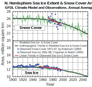
Analyses are ongoing to assess Southern Hemisphere sea ice changes, as well as changes in snow cover.
c. Multidecadal variability
Delworth and Mann (2000) have recently com-pared the simulated multidecadal variability in the North Atlantic of the R15 coupled model to a new multiproxy reconstruction of climate over the last several centuries. In both the model and proxy reconstructions the spec-trum of climate variability has a clear peak on the multidecadal time scale (approximately 60-80 years). The simulated variability involves fluctuations in the North Atlantic THC. A comparison of the spatial struc-tures between the model and the observations reveals relatively good agreement in the North Atlantic sector. Preliminary analyses with the R30 coupled model indi-cate that similar variability exists in the higher resolu-tion model. Such detailed comparisons of model and proxy data offer a promising pathway for increasing our understanding of decadal to centennial scale variability. Delworth and Greatbatch (2000) have also used the R15 model to demonstrate that such multidecadal variability of the THC is partially attributable to stochastic forcing of the ocean through the surface heat flux.
d. Extreme event in a 12,000 year coupled run
A control integration of one version of the R15 coupled model now has been extended beyond 12,000 years, thereby offering insights into centennial to millennial scales of variability. In this extended run a highly anomalous event occurs in the high latitudes of the North Atlantic at approximately model year 3100. A large pulse of fresh water, originating in the Arctic, moves southward through the Fram Strait into the North Atlan-tic. This fresh water pulse is accompanied by reduced oceanic convection and cold surface air temperature (an-nual mean anomalies of -4 K, corresponding to 6 stand-ard deviations below the mean). This event appears to be an extremely high amplitude realization of a promi-nent mode of internal variability of the coupled system (Delworth et al., 1997). Investigations of the dynamics of this variability are ongoing.
4. Simulation of the Ice Age - implications for cli-mate sensitivity
A major source of uncertainty in climate model projections of future climate involves the sensitivity of the climate system to radiative forcing. One way to evalu-ate the realism of a model’s climevalu-ate sensitivity is to simu-late climates of the distant past where sufficient evidence exists to estimate the changes in climate forcing and re-sponse. In pursuit of this goal, Broccoli (2000) used a atmosphere-mixed layer ocean model, whose
atmos-pheric component is nearly identical to the one employed in the R30 coupled model, to examine the changes in tropical climate induced by the relatively well-docu-mented changes in radiative forcing that occurred 21,000 years ago during the last glacial maximum. At this time, continental ice sheets were greatly expanded, atmos-pheric CO2 was reduced by approximately 25%, and sea
level was more than 100 m lower. When incorporated into the climate model, these changes produced a mean cooling of 2 K for the region from 30oS to 30oN.
Comparison of this simulated cooling with a vari-ety of paleodata indicates that the overall tropical cool-ing is comparable to paleoceanographic reconstructions based on alkenones and species abundances of plank-tonic microorganisms, but smaller than the cooling in-ferred from noble gases in aquifers, pollen, snow line depression, and the isotopic composition of corals. The paucity of paleoclimatic evidence for tropical cooling smaller than that simulated by the model suggests that it is unlikely that the model exaggerates the actual climate sensitivity in the tropics. A more definitive evaluation of the realism of the tropical sensitivity of the model must await the resolution of the differences in the mag-nitude of tropical cooling reconstructed from the vari-ous paleoclimatic proxies.
5. Future plans
and sharing most physics modules with future climate models.
The development of a new climate model for use in long control integrations, global warming scenario generation, and paleoclimatic studies is currently focused on a T42 resolution spectral atmosphere coupled to an ocean model with 2o horizontal resolution, except in the
tropics where finer resolution is retained to provide a better ENSO simulation. An ice model with viscous-plas-tic rheology will also be incorporated. A 1o version of
the ocean model is also undergoing initial testing. At present, the oceanic, land, and ice components are closer to being finalized than the atmospheric component. Plans also involve using both grid and spectral atmospheric models, at resolutions of T106 and higher, coupled to mixed layers or with fixed SSTs (or SSTs generated in lower resolution coupled model global warming scenario studies) to evaluate how alternative atmospheric physi-cal packages affect climate sensitivity and regional cli-mate change.
References
Broccoli, A.J., 2000: Tropical cooling at the last glacial maximum: An atmosphere-mixed layer ocean model simulation. J. Climate, in press.
Chapman, W.L., and J.E. Walsh, 1993: Recent variations of sea ice and air temperature in high latitudes. Bull. Amer.
Meteor. Soc., 74, 33-47.
Delworth, T.L., S. Manabe, and R.J. Stouffer, 1997: Multidecadal climate variability in the Greenland Sea and surrounding regions: a coupled model simulation.
Geophys. Res. Lett., 24, 257-260.
Delworth, T.L., and M.E. Mann, 2000: Observed and simulated multidecadal variability in the Northern Hemi-sphere. Climate Dynamics, accepted.
Delworth,T.L., and R.E. Greatbatch, 2000: Multidecadal thermohaline circulation variability driven by atmos-pheric surface flux forcing, J. Climate, in press.
Dixon, K.W., and J. Lanzante, 1999: Global mean sur-face air temperature and North Atlantic overturning in a coupled GCM climate change experiment. Geophys. Res.
Lett., 26, 2749-2752.
Dixon, K.W., T.L. Delworth, M. Spelman, and R.J. Stouffer,1999: The influence of transient surface fluxes on North Atlantic overturning in a suite of coupled GCM climate change experiments. Geophys. Res. Lett., 26, 1885-1888.
Haywood, J.M., R.J. Stouffer, R.T. Wetherald, S. Manabe, and V. Ramaswamy,1997: Transient response of a cou-pled model to estimated changes in greenhouse gas and sulfate concentrations. Geophys. Res. Lett., 24, 1335.
Jones, P.D., 1994: Hemispheric surface air temperature variations: a reanalysis and an update to 1993. J.
Cli-mate, 7, 1794-1802.
Kattenberg, A., et al. in Climate Change 1995: The
Sci-ence of Climate Change (eds. J. Houghton et al.)
285-357 (Cambridge Univ. Press, 1996).
Knutson, T.R., T.L. Delworth, K.W. Dixon, and R.J. Stouffer, 1999: Model assessment of regional surface tem-perature trends (1949-97). J. Geophys. Res., in press.
Mitchell, J.F.B., T.C. Johns, J.M. Gregory, S.F.B. Tett, 1995: Climate response to increasing levels of greenhouse gases and sulfate aerosols. Nature, 376, 501.
Parker, D.E., C.K. Folland, and M. Jackson, 1995: Ma-rine surface temperature: observed variations and data requirements. Clim. Change, 31, 559-600.
Robinson, D. A., 1993: Hemispheric snow cover from satellites. Ann. Glaciol., 17, 367-371.
Vinnikov, K.Y., A. Robock, R.J. Stouffer, J.E. Walsh, C.L. Parkinson, D.J. Cavalieri, J.F.B. Mitchell, D. Garrett, and V.F. Zakharov, 1999: Detection and attribution of global warming using Northern Hemisphere sea ice. Science, in press.
Wetherald,R.E., and S. Manabe, 1999: Detectability of summer dryness caused by greenhouse warming. Climatic
-6 -5
-4 -3
-2 -1
0 1
2 3
4 5
6 20E 40E 60E 80E 100E 120E 140E 160E 40S
20S EQ 20N 40N
2.5
60E 80E 100E 120E 20S
EQ 20N 40N
AIR Composite
A B
-6 -5
-4 -3
-2 -1
0 1
2 3
4 5
6 20E 40E 60E 80E 100E 120E 140E 160E 40S
20S EQ 20N 40N
0.1
60E 80E 100E 120E 20S
EQ 20N 40N
EOF-4 8.0%
[image:19.595.132.459.77.335.2]C D
Fig. 2: The composite difference of seasonally averaged (a) 850hPa wind (unit vector=2.5ms-1
) and (b)
precipita-tion anomalies (mm day-1
) for years of above normal all-India rainfall versus years of below normal all-India rainfall (see Fig. 1). (c) The fourth mode of variability extracted from an empirical orthogonal function analysis of seasonal anomalies of 850hPa wind. The magnitude of the wind anomalies is the product of the principal
compo-nent time series and the compocompo-nents of the wind. Typical variations of this mode are 1-2ms-1
. (d) precipitation anomalies (mm day-1) constructed from the difference of composites based on years when the principal component time series of mode 4 was of above normal versus below normal using +/-0.5 standard deviations thresholds.
Jun 1 Jul 1 Aug 1 Sep 1
1987 -100
-50 0 50 100
% Normal / PC-3
AIR PC-3
R=0.59
-4.0 -2.0 0.0 2.0 4.0
Standard Deviations 0.00
0.02 0.04 0.06 0.08 0.10
Probability
PDF NCEP/NCAR 850hPa uv PC-3
June-September (daily) 1958-97
All Years (+) AIR (-) AIR
-9 -7.5
-6 -4.5
-3 -1.5
0 1.5
3 4.5
6 7.5
9 20E 40E 60E 80E 100E 120E 140E 160E 40S
20S EQ 20N 40N
0.1
60E 80E 100E 120E 20S
EQ 20N 40N
EOF-3 6.6%
A B
C D
Fig. 3: (a) The third mode of variability extracted from an empirical orthogonal function analysis of daily anoma-lies of 850hPa wind. Typical variations of this mode are 2-4ms-1. (b) precipitation anomalies (mm day-1) constructed
from the difference of composites based on days when the principal component of mode 3 was of above normal versus below normal using +/-1 standard deviations thresholds. (c) Observed daily all-India rainfall (filled curve, expressed as a percentage of normal) and the principal component time series of mode 3 (red line) for 1987. Both time series have been smoothed with a 5-day running mean. (d) Probability distribution functions of the principal component time series of mode 3 for all years (black line), years of above normal all-India rainfall (green line) and below normal all-India rainfall (red line). The years of above normal and below normal all-India rainfall are given
[image:19.595.137.463.427.679.2]1865
1890
1915
1940
1965
1990
2015
2040
0.4
0.2
0
0.2
0.4
0.6
0.8
1
1.2
1.4
1.6
1.8
2
T
emperature (K)
Global Mean Temperature
Experiment 1
Experiment 2
Experiment 3
Experiment 4
Experiment 5
Observations
N. Hemisphere Sea Ice Extent & Snow Cover Area
GFDL Climate Model and Observations. Annual Averages
1900 1920 1940 1960 1980 2000 2020 2040
Year
10
12
14
16
18
20
22
24
26
28
Area, million square km
Modeled Sea Ice & Snow Cover
Anthropogenic Trends in Modeled Sea Ice & Snow Cover
Observed Sea Ice 1901-98, Chapman & Walsh (1993) Observed Snow Cover 1971-97, by Robinson (1993)
Linear Trends in Observed Sea Ice & Snow Cover
[image:20.595.95.490.63.333.2]Sea Ice
Snow Cover
Fig. 1: Time series of observed (heavy black line) and simulated (various thin colored lines) global mean surface temperature over the period 1865 to 2040 (1997 for the observations). The simulated lines are from 5 independent realizations of the GFDL R30 coupled model forced with estimates of observed greenhouse gases and sulfate aerosols until 1990, and projections thereafter. The model output is sampled only for those locations and times at which obser-vational data exist. For both model and observations, surface air temperature is used over the continents, while sea surface temperature is used over the oceans. The observed data are a combination of the Jones (1994) surface air temperature data and the Parker et al. (1995) sea surface temperature, updated through 1997. Anomalies are plotted relative to the 1880-1920 mean for both the model and observations.
Fig. 2: Observed and simulated time series of Northern Hemisphere sea ice extent and snow cover (after Vinnikov et al.,1999).
[image:20.595.136.440.448.736.2]Climate Variability at Decadal and Interdecadal Time Scales
Dörthe Handorf1
, Vladimir K. Petoukhov2
, Klaus Dethloff1, Alexey V. Eliseev2
, Antje Weisheimer,
Igor I. Mokhov2
1Alfred Wegener Institute for Polar and Marine Research, Research Department Potsdam,
Telegrafenberg A 43, D-14473 Potsdam, Germany
2Obukhov Institute of Atmospheric Physics of Russian Academy of Sciences,
Pyzhevsky 3, 109017 Moscow, Russia
corresponding e-mail: [email protected]
O
nly with an improved understanding of natural mate variability confident estimations of possible cli-matic changes due to anthropogenic influences can be given. In view of the observed