Genetic Algorithm Optimization for Blind Channel
Identification with Higher Order Cumulant Fitting
S. Chen, Y. Wu, and S. McLaughlin
Abstract—An important family of blind equalization algorithms
identify a communication channel model based on fitting higher order cumulants, which poses a nonlinear optimization prob-lem. Since higher order cumulant-based criteria are multimodal, conventional gradient search techniques require a good initial estimate to avoid converging to local minima. We present a novel scheme which uses genetic algorithms to optimize the cumulant fitting cost function. A microgenetic algorithm implementation is adopted to further enhance computational efficiency. As is demonstrated in computer simulation, this scheme is robust and accurate and has a fast convergence performance.
Index Terms— Blind channel identification, genetic algorithm,
higher order cumulant fitting.
I. INTRODUCTION
M
ANY digital communication channels are subject to in-tersymbol interference (ISI) [1]–[3]. The ISI distortion of a channel is due to the restricted bandwidth allocated to the channel or the presence of multipath effects in the transmission medium. At the receiver, the ISI must be compensated to reconstruct the transmitted data symbols, and this is referred to as channel equalization. Traditionally, an equalizer learns the channel characteristics through an initial training period. During training, the transmitter sends out a data sequence that is known and available in proper synchronism at the receiver. The receiver uses this sequence as the desired reference signal to adjust the equalizer parameters. Once the channel char-acteristics have been learned sufficiently well, the equalizer can then switch to a decision-directed mode with the detected symbol sequence serving as the reference signal. This decision-directed adaptation allows an equalizer to track slow variations in the channel characteristics during actual data transmission. Training consumes valuable bandwidth resource and should be avoided whenever possible. Furthermore, in multipoint broadcast communication systems, it is impossible to have a training period, and an equalizer must adjust itself based only on noisy channel observations without access to the desired reference. This is known as blind equalization. Blind equalization techniques developed since the pioneering work of Sato [4] can be categorized into three classes that either rely on: 1) Bussgang-type techniques [4]–[9]; 2) higher order cu-mulants (HOC’s) or equivalent higher order spectra [10]–[15]; or 3) a joint channel and data estimation approach [16]–[21].Manuscript received November 4, 1996; revised May 16, 1997, November 26, 1997, and December 15, 1997.
S. Chen and Y. Wu are with the Department of Electrical and Electronic Engineering, University of Portsmouth, Portsmouth PO1 3DJ U.K.
S. McLaughlin is with the Department of Electrical Engineering, University of Edinburgh, Edinburgh EH9 3JL U.K.
Publisher Item Identifier S 1089-778X(97)09409-5.
Blind equalizers based on HOC techniques are very general and often achieve excellent practical results, provided that sufficient signal samples are available to accurately estimate higher order statistics.
For the second family of blind equalizers, a two-stage strategy is usually adopted, which first identifies a channel model using HOC fitting algorithms and then employs the estimated channel model to design an equalizer [14], [15]. The key step of this approach is its ability to obtain an accurate channel model. Once this model is available, a variety of existing equalizer design methods can be employed, ranging from a simple linear inverse filter to a sophisticated maximum likelihood sequence estimator [1], [22]–[24], depending on a tradeoff between performance and complexity. HOC fitting algorithms for blind channel identification are widely used in practice due to their simplicity and computational efficiency.
Cost functions of HOC fitting, however, are multimodal, and conventional gradient optimization techniques [14], [15] may converge to “wrong” solutions unless a good initial value for the channel parameters is provided, which is not always possible. To overcome the problem of local minima, simulated annealing (SA) has been implemented to optimize the HOC fitting cost function [25]. Here we propose genetic algorithms (GA’s) [26]–[31] for blind channel identification based on HOC fitting. For this particular application, we believe that the GA approach is more efficient than SA. Our simulation study demonstrates that the GA-based scheme is robust to errors in estimated HOC’s and can achieve a global optimal solution regardless of initial value of channel estimate. Furthermore, the number of parameters to be optimized in the problem of blind channel estimation is usually small, and GA’s are particularly effective for this kind of optimization problems. The micro-GA GA) implementation [30] is adopted in our scheme to further improve the convergence rate.
II. BACKGROUND
Typically, a digital communication channel can be modeled as a finite impulse response filter (also known as a mov-ing average model) with an additive noise source [1]–[3]. Specifically, the received signal at sample is given by
(1)
where denotes the noiseless channel output, is the channel order, are the channel taps, the symbol sequence is independent and identically distributed, and is a Gaussian white noise sequence with zero mean and variance We assume that the channel and symbols
are real valued. This corresponds to the use of a multilevel pulse amplitude modulation -PAM) scheme with a symbol constellation defined by the set
(2)
For example, an 8-PAM scheme has a data symbol set { 7, 5, 3, 1, 1, 3, 5, 7}. Extension to complex-valued channels and modulation schemes is straightforward. The reason for concentrating on the simpler real-valued case is to avoid com-plicated communication terminologies, which some readers might not be familiar with.
In the ideal situation where the ISI is absent, the received signal is given by
(3)
The optimal decision process in this case is trivial and can readily be shown to be
(4)
where denotes the estimate of The ISI
distortion refers to the fact that, in reality, the received signal is a mixture of several transmitted data symbols. Even without noise, the threshold decision rule (4) is no longer reliable because data symbols transmitted before and after will interfere with the decision regarding the transmitted symbol
If the channel model
(5)
is known, this ISI distortion can be removed or minimized by employing an equalizer. Equalizer design given a known channel model is a well-developed field, and a variety of techniques are available [1], [22]–[24]. The channel model is generally unknown, however, and has to be identified first. Blind channel identification refers to the determination of the channel model using only the noisy received signal and some prior knowledge of statistical properties of The problem is particularly difficult because the transfer function of the channel
(6)
is generally nonminimum phase. is said to be minimum phase if all the zeros of are inside the unit circle of the -plane. If has zeros outside the unit circle, it is non-minimum phase. For nonnon-minimum phase channels, methods based on second-order statistics fail to work completely, and higher order statistics have to be employed. The second-order cumulant or autocorrelation function of the received channel output sequence is well known to be
(7)
where is the symbol variance and
and for The fourth-order cumulant sequence
of is defined as
(8)
It can be shown that [32]
(9)
where
(10)
and
(11)
is the kurtosis of the transmitted symbol sequence
The four-order cumulant is considered because third-order cumulants of symmetric sequences are zero. The variance and the kurtosis are known in our application.
As is well known, the autocorrelation functions do not carry any phase information but the HOC’s are very sensitive to phase properties. The frequency response of the transfer function is defined by
(12)
where is the amplitude response and is the
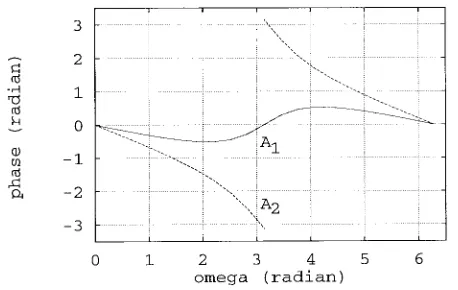
phase response. Consider the simplest case with
Assume that we have two transfer functions defined by
and (13)
where is minimum phase since its zero
is inside the unit circle, and is nonminimum phase as its zero is outside the unit circle. Both have the
same amplitude response but very different
Fig. 1. Phase responses of A1(z) = 1:0 + 0:5z01 and A2(z) = 0:5
+ 1:0z01.
TABLE I
A COMPARISON OFCUMULANTS ANDAUTOCORRELATIONS FOR
A(z) = a0+ a1z01 WITHa0= 1:0; a1= 0:5 (MINIMUM
PHASE)ANDa0= 0:5; a1= 1:0 (NONMINIMUMPHASE). THE
RECEIVEDCHANNELOUTPUTISr(k): AUTOCORRELATION
FUNCTIONSLOSE THEPHASEINFORMATION OF THESIGNAL
HOC’s are insensitive to Gaussian noise. This can readily be verified by comparing (9) with (7).
Assume that received signal samples are used to compute the time estimate of the fourth-order cumulant. is obtained by replacing the moments in (8) with their respective sample averages based on the samples of The optimal channel estimate can be obtained by minimizing the following cumulant-fitting cost function [15], [25]:
(14)
In the construction of the fourth-order cumulant-based cost function (14), only the diagonal slice of is used as this results in much reduced computational complexity. Moreover, it has been found in practice that fitting cumulants over their entire region of support does not give any significant improvement in channel model estimation. It is obvious that the accuracy of the estimated cumulant will influence the result of this approach. To reduce the estimation variance of the segment-average scheme [11]
is often used to compute In this approach,
blind channel estimation is formulated as a standard optimiza-tion problem with the cost funcoptimiza-tion This is attractive since the concepts and principles of the related optimization are widely understood.
With the exception of [25], existing algorithms for HOC fitting employ gradient search techniques, yet the associated cost functions are well known to be multimodal. Even with
measures of providing good initial channel estimates, it has been observed that gradient algorithms sometimes converge to local minima [14]. Using GA’s to optimize the cost function (14) has the advantage of ensuring a global optimal channel estimate in the limit. Moreover, a communication channel model (5) typically contains a few tap coefficients. Thus the number of parameters to be optimized in (14) is small, and GA’s are often very efficient in solving this kind of “small-dimensional” optimization problems. We also discovered in simulation that GA’s are less sensitive to noisy errors in the time estimate of
In reality, the channel order is unknown and needs to be identified. Several model-order selection criteria can be applied to determine the correct order [32]–[34], and they will not be repeated here. This model-order selection process will add considerably more computational complexity. A much simpler method is to overfit with an upper bound Thus the cost function used in the optimization process is modified as
(15)
Function (15) is more complicated than (14) because it con-tains more local minima, and this will generally cause more problems for gradient-based methods. The GA-based method, however, should in principle be capable of identifying those nonexisting taps with (near) zero values, since the true global optimal values for nonexisting taps are zeros. This has been confirmed in simulation. An inspection of the obtained channel estimate will allow deleting those insignificant taps. Thus, the proposed method has an additional advantage of much simpler model-order selection.
III. METHOD
With the goal being to find a global optimum solution as quickly as possible, we adopt the so-called GA [30], which appears to offer certain advantages. This version of GA uses a population that is much smaller than typically employed, which can make it less computationally burdensome. In [30], it was reported that the GA can find optimal regions faster than standard GA’s for selected optimization problems. Allowing a single sequence of a GA to converge, however, may not be very useful apart from quickly locating local optima. There-fore, after such convergence, the population is reinitialized randomly while the best individual found up to that point is copied into the newly generated population. This iterative reinitialization is repeated until no further improvement is evidenced.
points typically set to four. No mutation is employed, as the reinitialization routine serves to introduce diversity. Tour-nament selection [30] is employed to determine parents for reproduction.
More specifically, the procedure is summarized as follows. Step 1) Given a set of received signal samples
assume an overlength and compute the re-quired time estimate of the fourth-order cumulant,
for to form the
cumulant fitting cost function (15).
Step 2) With a set of randomly initialized channel param-eter vectors where is the population size, use the GA to optimize the cost function (15). The fitness function value corresponding to is defined as
(16)
In the case that is (near) zero, a very large value is assigned to . The operation of the GA involves two loops.
Step 2.1) The inner loop evaluates and evolves a pop-ulation. Let be the best fitness value of the current population. The population is assumed to have converged if
(17)
where is a predefined small positive con-stant.
Step 2.2) After the convergence of the inner loop, the convergence of the outer loop is tested. Let be the best channel estimate in the cur-rent population and be the best channel estimate recorded in the previous population. The overall process has converged if
(18)
where the small positive scalar defines the
final search accuracy, and is
the Euclidean norm of the search space (as the search range for each parameter is [ 1, 1]). Otherwise, the population is reinitialized,
is reset to and the inner
loop restarts.
To increase the chance of converging to a true global optimum solution, a more robust outer loop test can be employed which only terminates the overall process after the test (18) has been satisfied for several consecutive times.
A “normalization” measure is developed from (9) to im-prove the rate of convergence. We make sure that every candidate satisfies
(19)
where is the th element of In the population ini-tialization, the taps of each channel vector first take values randomly from the interval ( 1, 1), and each chosen model is then normalized according to (19). Whenever a new generation is produced, each member of the population is also normalized. This ensures that each member of the population is inside the feasible set of channel models. Without this normalization measure, mating will inevitably produce some population members that are far outside the possible set of candidate channel models, and function evaluations for these members will merely waste computation.
It is well known that sign and time-shift ambiguities exist in blind channel identification based on HOC fitting. Sign ambiguity is manifested by the fact that both the true channel and are global optimal solutions of (15) [or (14)]. Time-shift ambiguity can be illustrated in the following example.
Let the true channel model be with
and Suppose that is
used. Then and
are all global optimal solutions of (15). These “ambiguity” problems are common to blind equalization techniques. A solution to time-shift ambiguity is to fix one of the channel coefficients. We do not fix a tap value but instead check if the first tap of a population member is zero (absolute value smaller than a threshold), and if so, a shifting is performed to ensure that the first tap is always nonzero.
In practice, the convergence performance of the algorithm can only be observed through the best value of the cost function In simulation, the performance of the algorithm can also be assessed by the following mean tap error (MTE)
(20)
where with for is the true channel. In (20),
is used if converges to otherwise is
used. This is necessary as both and are correct global optimal channel estimates for HOC fitting cost functions (see the above discussion on sign ambiguity).
IV. RESULTS
Simulation was conducted to test the proposed scheme using two channels taken from [2]. The impulse response of these two channels are given by
Channel 1 Channel 2
(21)
respectively. There were 8-PAM data symbols transmitted, and 50 000 noisy received data samples were used to compute the time estimate of the fourth-order cumulant. The signal-to-noise ratio (SNR) in the simulation was defined as
(22)
(a)
[image:5.612.346.517.55.304.2](b)
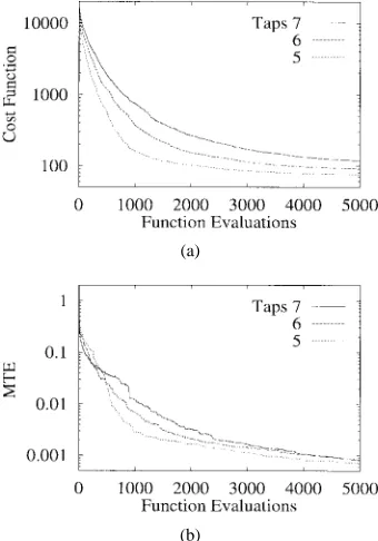
Fig. 2. (a) Cost function and (b) MTE versus number of function evaluations averaged over 100 different runs. Channel 1, 8-PAM, and SNR= 20 dB.
(a)
(b)
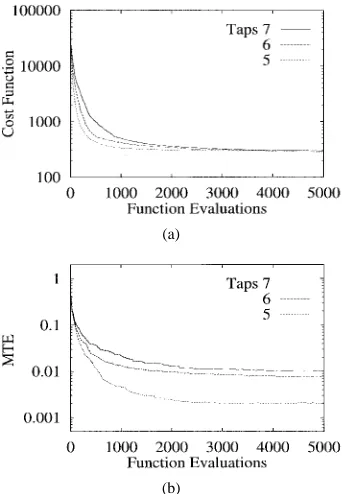
Fig. 3. (a) Cost function and (b) MTE versus number of function evaluations averaged over 100 different runs. Channel 1, 8-PAM, and SNR= 30 dB.
Figs. 2–4 depict evolutions of the cost function
and the MTE for channel 1 with different SNR conditions and assumed channel lengths respectively. Tables II and III summarize the blind identification results (mean standard deviation) for channel 1 with SNR’s of 20 and 40 dB, respectively. Simulation results for channel 2 are similarly given in Figs. 5–7 and Tables IV and V. It is well known that channel 2 is much more difficult to equalize than channel 1, and this was reflected in terms of accuracy in our simulation results.
(a)
(b)
[image:5.612.84.256.58.305.2] [image:5.612.83.253.347.590.2]Fig. 4. (a) Cost function and (b) MTE versus number of function evaluations averaged over 100 different runs. Channel 1, 8-PAM, and SNR= 40 dB.
TABLE II
[image:5.612.307.554.504.593.2]IDENTIFICATIONRESULTS FORCHANNEL1WITH8-PAMANDSNR= 20 dB
TABLE III
IDENTIFICATIONRESULTS FORCHANNEL1WITH8-PAMANDSNR= 40 dB
(a)
[image:6.612.84.256.57.306.2](b)
Fig. 5. (a) Cost function and (b) MTE versus number of function evaluations averaged over 100 different runs. Channel 2, 8-PAM, and SNR= 20 dB.
(a)
(b)
Fig. 6. (a) Cost function and (b) MTE versus number of function evaluations averaged over 100 different runs. Channel 2, 8-PAM, and SNR= 30 dB.
of function evaluations for the scheme was typically a few thousand, as confirmed in Figs. 2–7.
V. DISCUSSION
Some observations can readily be drawn from the simulation results. In the simulation, the GA-based scheme always converged close to a global optimal channel estimate and the optimization process converged quickly. Compared with other existing methods of HOC fitting, the method appears
(a)
(b)
[image:6.612.346.517.58.305.2]Fig. 7. (a) Cost function and (b) MTE versus number of function evaluations averaged over 100 different runs. Channel 2, 8-PAM, and SNR= 40 dB.
TABLE IV
IDENTIFICATIONRESULTS FORCHANNEL2WITH8-PAMANDSNR= 20 dB
TABLE V
IDENTIFICATIONRESULTS FORCHANNEL2WITH8-PAMANDSNR= 40 dB
TABLE VI
COMPUTATIONALCOMPLEXITY OF THEPROPOSEDGA. NgIS THE
NUMBER OFGENERATIONS FOR THEALGORITHM TOCONVERGE,N IS THE
NUMBER OFSAMPLES,AND^naIS THEASSUMEDCHANNELLENGTH
[image:6.612.82.255.349.595.2]data symbols and reducing the length of data samples for cumulant computation to 20 000. The results, not shown, are similar to those reported here. For other existing methods of HOC fitting, it is common that estimation accuracy will reduce and estimation variance will increase as SNR decreases. For the GA-based method, the simulation results suggest that, at least for the two channels tested, SNR has little effect on convergence rate and estimation accuracy. As was expected, our method is capable of identifying nonexisting channel taps with (near) zero values (at least an order smaller than values for existing taps). This is particularly important when an overlengthed channel model is used to avoid time-consuming model-order selection.
For this particular application, the convergence rate of the GA-based scheme is faster than that of the SA-based scheme reported in [25]. All the HOC-fitting algorithms have the same requirements of cumulant computation. Since the computational complexity per function evaluation is similar for GA and SA, we can compare their complexity by their required numbers of function evaluations. The number of function evaluations required for the GA scheme to converge was typically a few thousand in the simulation. This is compared favorably with the SA scheme. The number of function evaluations for the SA algorithm of [25] is
where and are the lengths of the two loops for step adjustment and is the number of “temperature reductions.” Quoting the figures from [25] with
and the required number of
function evaluations for the channels used in our simulation study would nearly be 30 000.
REFERENCES
[1] S. U. H. Qureshi, “Adaptive equalization,” Proc. IEEE, vol. 73, pp. 1349–1387, Sept. 1985.
[2] J. G. Proakis, Digital Communications. New York: McGraw-Hill, 1983.
[3] C. F. N. Cowan and P. M. Grant, Adaptive Filters. Englewood Cliffs, NJ: Prentice-Hall, 1985.
[4] Y. Sato, “A method of self-recovering equalization for multilevel amplitude-modulation systems,” IEEE Trans. Commun., vol. COM-23, pp. 679–682, 1975.
[5] D. Godard, “Self-recovering equalization and carrier tracking in two-dimensional data communication systems,” IEEE Trans. Commun., vol. COM-28, pp. 1867–1875, 1980.
[6] J. R. Treichler and B. G. Agee, “A new approach to multipath correction of constant modulus signals,” IEEE Trans. Acoust., Speech, Signal Processing, vol. ASSP-31, no. 2, pp. 459–472, 1983.
[7] G. Picchi and G. Prati, “Blind equalization and carrier recovering using a stop-and-go decision-directed algorithm,” IEEE Trans. Commun., vol. COM-35, pp. 877–887, 1987.
[8] N. K. Jablon, “Joint blind equalization, carrier recovery, and timing recovery for high-order QAM signal constellations,” IEEE Trans. Signal Processing, vol. 40, pp. 1383–1398, June 1992.
[9] S. Chen, S. McLaughlin, P. M. Grant, and B. Mulgrew, “Multi-stage blind clustering equalizer,” IEEE Trans. Commun., vol. 43, no. 3, pp. 701–705, 1995.
[10] K. S. Lii and M. Rosenblatt, “Deconvolution and estimation of transfer function phase and coefficients for non-Gaussian linear processes,” Ann. Statist., vol. 10, pp. 1195–1208, 1982.
[11] G. B. Giannakis and J. M. Mendel, “Identification of nonminimum phase system using higher order statistics,” IEEE Trans. Acoust., Speech, Signal Processing, vol. 37, pp. 360–377, 1989.
[12] H.-H. Chiang and C. L. Nikias, “Adaptive deconvolution and identifi-cation of nonminimum phase FIR systems based on cumulants,” IEEE Trans. Automat. Contr., vol. 35, pp. 36–47, 1990.
[13] D. Hatzinakos and C. L. Nikias, “Blind equalization using a tricepstrum-based algorithm,” IEEE Trans. Commun., vol. 39, pp. 669–682, May 1991.
[14] F.-C. Zheng, S. McLaughlin, and B. Mulgrew, “Blind equalization of nonminimum phase channels: Higher order cumulant based algorithm,” IEEE Trans. Signal Processing, vol. 41, pp. 681–691, Feb. 1993. [15] J. K. Tugnait, “Blind equalization and estimation of digital
communi-cation FIR channels using cumulant matching,” IEEE Trans. Commun., vol. 43, no. 2/3/4, pp. 1240–1245, 1995.
[16] M. Ghosh and C. L. Weber, “Maximum-likelihood blind equalization,” in Proc. SPIE, vol. 1565, pp. 188–195, San Diego, CA, 1991. [17] N. Seshadri, “Joint data and channel estimation using blind trellis search
techniques,” IEEE Trans. Commun., vol. 42, no. 2/3/4, pp. 1000–1011, 1994.
[18] K. Giridhar, J. J. Shynk, and R. A. Iltis, “A modified Bayesian algorithm with decision feedback for blind adaptive equalization,” in Preprints 4th IFAC Int. Symposium Adaptive Systems in Control and Signal Processing, France, 1992, pp. 737–742.
[19] E. Zervas, J. Proakis, and V. Eyuboglu, “A quantized channel approach to blind equalization,” in Proc. ICC’92, Chicago, 1992, vol. 3, pp. 351.8.1–351.8.5.
[20] J. G. Proakis, “Adaptive algorithms for blind channel equalization,” in Proc. 3rd IMA Conf. Mathematics Signal Processing, Univ. of Warwick, U.K., 1992.
[21] S. Chen and Y. Wu, “Maximum likelihood joint channel and data estimation using genetic algorithms,” IEEE Trans. Signal Processing, vol. 46, pp. 1469–1473, May 1998.
[22] D. Williamson, R. A. Kennedy, and G. W. Pulford, “Block decision feedback equalization,” IEEE Trans. Commun., vol. 40, pp. 255–264, Feb. 1992.
[23] S. Chen, B. Mulgrew, and S. McLaughlin, “Adaptive Bayesian equalizer with decision feedback,” IEEE Trans. Signal Processing, vol. 41, pp. 2918–2927, Sept. 1993.
[24] G. D. Forney, “Maximum-likelihood sequence estimation of digital sequences in the presence of intersymbol interference,” IEEE Trans. Inform. Theory, vol. IT-18, no. 3, pp. 363–378, 1972.
[25] J. Ilow, D. Hatzinakos, and A. N. Venetsanopoulos, “Blind equaliz-ers with simulated annealing optimization for digital communication systems,” Int. J. Adapt. Contr. Signal Process., vol. 8, pp. 501–522, 1994.
[26] J. H. Holland, Adaptation in Natural and Artificial Systems. Ann Arbor, MI: Univ. of Michigan Press, 1975.
[27] D. E. Goldberg, Genetic Algorithms in Search, Optimization, and Ma-chine Learning. Reading, MA.: Addison-Wesley, 1989.
[28] J. J. Grefenstette, “Optimization of control parameters for genetic algorithms,” IEEE Trans. Syst. Man. Cybern., vol. SMC-16, no. 1, pp. 122–128, 1986.
[29] L. Davis, Ed., Handbook of Genetic Algorithms. New York: Van Nostrand Reinhold, 1991.
[30] K. Krishnakumar, “Micro-genetic algorithms for stationary and nonsta-tionary function optimization,” in Proc. SPIE Intell. Cont. Adapt. Syst., vol. 1196, pp. 289–296, 1989.
[31] L. Yao and W. A. Sethares, “Nonlinear parameter estimation via the genetic algorithm,” IEEE Trans. Signal Processing, vol. 42, pp. 927–935, Apr. 1994.
[32] J. M. Mendel, “Tutorial on higher-order statistics (spectra) in signal pro-cessing and system theory: Theoretical results and some applications,” Proc. IEEE, vol. 79, pp. 278–305, Mar. 1991.
[33] G. B. Giannakis and J. M. Mendel, “Cumulant-based order determi-nation of non-Gaussian ARMA models,” IEEE Trans. Acoust., Speech, Signal Processing, vol. 38, pp. 1411–1423, Aug. 1990.