The elasto-mechanical behaviour of Douglas fir, its sensitivity to tree-specific properties, wind and snow loads, and implications for stability – a simulation study

JOURNAL OF FOREST SCIENCE, 48, 2002 (2): 49–69

The stability of single trees and of entire forest stands against wind-induced damage, such as stem breakage and uprooting, has been an intensely studied subject for many years (e. g., BARGMANN 1904). Recent storm disasters gave rise to an integrated, international expert exchange (conference on wind and wind-related damage to trees in Edinburgh, 1993: COUTTS, GRACE 1995; conference on wind and other abiotic risks to forests in Joensuu, 1998: PELTOLA 2000). One outcome is a stand risk simulator, freely accessible on the Internet* _{(“STORMS project} dem-onstrator”: MILLER et al. 2000). Uniting different models that account for the relations between wind forces and the mechanical reactions of trees (ForestGALES: QUINE

1998; GARDINER, QUINE 2000); HWIND: PELTOLA et al. 1999; TALKKARI et al. 2000; and models of VALINGER

and FRIDMAN (1997; FRIDMAN, VALINGER 1998), the risk either of breakage or turn-over can be estimated in depen-dence on site-, stand- and tree-related characteristics, which will allow deriving damage preventive decisions.

Apart from economically based management interests in the mechanical failure of trees, mechanical aspects are also of fundamental biological concern, especially the physical properties of the stem which highly contribute to the ability of a tree to come out on top against its

competitors (MOSBRUGGER 1990; NIKLAS 1992). Further, plants can change their mechanical properties in the course of their ontogenetic development in order to cope best with the particular prevailing living conditions (SPECK 1994; SPECK et al. 1996; STERCK, BONGERS 1998). Aspects of mechanical stability and approaches to quan-tify and evaluate the safety of trees have been widely discussed (MCMAHON, KRONAUER 1976; KING, LOUCKS

1978; KING 1986; MATTHECK 1991; NIKLAS 1994; NI

-KLAS, SPATZ 1999), and hypotheses of adaptive growth and of stress and strain constancy of a stem bent by wind forces were set up (METZGER 1893; TIRÉN 1928; YLINEN

1952; WILSON, ARCHER 1979; MATTHECK 1990). Basically, responses to questions on this subject are to be obtained by experimental work, e. g., by simultaneous-ly measuring wind speed and fibre strain at the surface of the bent stem (BLACKBURN 1997; BLACKBURN, GARDI

-NER 1997) or by destructively sampling the tree (NIKLAS, SPATZ 2000). As such work is by nature very laborious and often tedious, in this context, a versatile tool is desir-able for detailed modelling of the architecture and the mechanical properties of a tree, and to simulate its elasto-mechanical reactions caused by defined wind and gravi-tational forces. By modifying tree-related parameters or

The elasto-mechanical behaviour of Douglas fir, its sensitivity

to tree-specific properties, wind and snow loads, and implications

for stability – a simulation study

D. G

, O. K

1

University of Göttingen, Faculty of Forest Sciences and Forest Ecology, Institute of Forest Biometry

and Informatics, Göttingen, Germany

2

University of Göttingen, Faculty of Physics, Institute of Theoretical Physics, Göttingen,

Germany

ABSTRACT: A full 3-D model was developed to simulate the elasto-mechanical behaviour of trees subjected to wind and

gravitational forces with the aim of estimating the stress and strain distribution at the surface of the stem. The model was adapted to geometry and material properties of a 64-year old Douglas fir tree. The results are comparable, on the whole, with those of a finite element model of this tree. Original stem and crown data, as well as the applied forces, were modified manifold in order to study their importance on the change in fibre stress and thus, on the safety reserve against stem break-age.

Keywords: Douglas fir; elasto-mechanical model; stress; strain; safety reserve; stem breakage

50 J. FOR. SCI., 48, 2002 (2): 49–69

acting forces, an exhaustive study of the sensitivity on the observed effects, firstly, the experienced stresses and strains, can be performed.

As existing models usually show deficiencies in repre-senting naturally built trees and realistic acting loads, a basic demand is to take into account the inhomoge-neous distribution of the wood density and of the Young’s modulus within the stem, as well as a crown spa-tially resolved into (first-order) branches (FOURCAUD, LAC 1996) and wind forces distributed according to the crown sail area (SPATZ, BRÜCHERT 2000; NIKLAS, SPATZ

2000). Additionally, the form of the stem cross section should enter the model, as the contribution of the form of the stem to its flexural stiffness is of great importance (SPECK et al. 1990; NIKLAS 1992).

In compliance with these demands, in a first approach, the finite element method (FEM) was applied to model a 64-year old Douglas fir tree including the acting forces (GAFFREY et al. 2001). As this model type turned out to be unhandy to variously realise changes of input parame-ters for sensitivity studies and because of some model-inherent weaknesses, another differential equation approach was chosen, in which the object is “holistical-ly” defined (SLOBODA, GAFFREY 1999; GAFFREY 2000), contrary to the finite elementary formulation.

First, this paper introduces the underlying theory of elasto-mechanics especially adapted for a stem consid-ered to be a compound material with spatially inhomoge-neous material properties and with an irregular cross-section form, and gives the mathematical formula-tion of the differential equaformula-tion problem and its soluformula-tion. Secondly, as strain measurements during bending of the tree were not performed and thus, data for verifying the simulation results do not exist, it is tested – to exclude significant model bugs – whether the prognostications of the finite element model (FE model) coincide with those of the holistic model (which was named TREEFLEX). Third, referring to the results based on the original tree data and on a certain assumed wind profile, TREEFLEX was ap-plied to estimate and evaluate the effects on stress change by varying crown structure, stem form and stem material characteristics, wind profiles, and by additional loads.

MATERIAL AND METHODS

A 64-year old Douglas fir tree, 29.55 m in height and with a dbh of 34.2 cm (without bark), coming from a pure stand located at Esbeek in the southern Netherlands, was destructively sampled in order to measure and estimate respectively, the masses of stem, branches and needles, the crown structure and sailing areas, the inner stem ge-ometry and the spatial distribution of wood density and Young’s modulus within the stem. (Further four neigh-bouring trees were examined, but as data are not present-ed here, for details see SLOBODA and GAFFREY [1999; GAFFREY, SLOBODA 2001].) In order to calculate wind

forc-es, a typical storm condition was defined and a certain theoretical static wind profile assumed. The tree and load model which is based on these very data serves as a ref-erence when modifications of either tree-specific or wind-related parameters are made. (Some data and illustrative demonstrations have been published on the Internet,** which will be indicated in the following.)

STEM GEOMETRY AND WOOD PROPERTIES

A stem analysis was performed by exactly digitising each year ring of 28 disks, the first one taken at a height of 0.4 m and the last at 27.0 m. In the model, 36 co-ordinates per ring, equidistantly spread, were used (data on the In-ternet). The total volume, excluding bark, was about 1.16 m3_.

Concerning the wood properties, it has to be stated that only the bulk density of oven-dry disks was actually measured. Thus, the estimated dry mass of the total stem was 639 kg and about 920 kg for fresh mass. As Douglas fir shows a typical, species-specific pattern of altering its wood density from ring to ring, starting with high values near the pith, a minimum at about the tenth year ring and an increase towards the peripheral rings, a corresponding density function was assumed to be valid for this tree, too, and was fitted for each stem disk (GAFFREY et al. 1999).

**_{http://www.uni.gaffrey.de (see page “Demos/Downloads”)}

It is ρ₈ (k,∆ρ_i) the wood density, at a moisture content of 8%, depending on the cambial age k, which is given by the ring number with the count beginning at the pith, and a shift term ∆ρ_i that accounts for the difference between disk-specific density and mean density. Regarding a spe-cific year ring, the wood density between two neighbour-ing stem disks was assumed to be constant. The density of the year ring in this section was calculated by averag-ing the raverag-ing-related densities of both disks, weighted by the cross-sectional areas of the rings. The density of fresh, green wood was estimated by assuming the moisture con-tent of the heartwood and sapwood, adopting mean liter-ature values, to be 30% and 120%, respectively, and to take account of the swelling. Due to modelling con-straints, instead of the real sapwood area, for all stem disks, the outer ten year rings were considered as the water-conducting rings.

Derived from the wood density was the modulus of elas-ticity (MOE) E*_{by applying published regression}

func-tions (PALKA 1973), in modification (GAFFREY et al. 1999).

8 2

6.33

( , ) 0.6

( 10) 69.86

i i

k

k

ρ ∆ρ = − + + ∆ρ

− + (g/cm3) (1)

(2)

E = E* ₍ρ

u. /ρ*u.)⋅[1 + a⋅∆u], ∆u = min[(u – u*], umax]

E* _{is the MOE at a reference density ρ}*

u. with moisture

content u*_{, a is –0.01 (PALKA 1973) and u}

Taken from literature (KOLLMANN 1951), for this Douglas fir tree, the MOE was assumed to be 11.5 GPa at a bulk density of 0.5 g/cm3 _{and at a moisture content of 12%.} Corrections for the moisture content of green wood were made.

Thus, due to the chosen model, the three-dimensional variation of the MOE follows that of the wood density. But it must be stated that this relation, though valid for Douglas fir in general, probably does not match the char-acteristics of this individual tree (NIKLAS 1997).

The finite element model of the stem (GAFFREY et al. 2001), too, is based on the data and assumptions de-scribed above, but some differences in geometry and wood properties must be outlined: each year ring is de-fined by only 16 co-ordinates, instead of 36, but the zones of heartwood and sapwood were modelled exactly as mea-sured, i. e., towards the stem base, the sapwood compris-es up to 25 year rings, in contrast to the fixed number of ten in TREEFLEX. In the FE model, density and Young’s modulus only differ between heartwood and sapwood and do not vary ring-wise. Lastly, the stem interval from 27.0 to 29.6 m was modelled in a different way: contrary to the real building of this section with finite elements, in TREEFLEX the stem ends at the position of the last stem disk at 27.0 m, and only the gravitational force exerted by the part above was added.

Simulation variants

The stem reference variant S_Ref is defined by the ge-ometry and the physical and mechanical properties which represent the stem of the investigated tree as exactly as possible by the given data. The following variant descrip-tions only account for divergences to the reference.

Stem geometry: In variant S_G1, instead of the geom-etry of the stem at the time of felling (which was after the end of the last growing season) the geometry prior to the last growing period is considered, i. e., the last year ring is omitted. Again, the ten (and not nine) outermost year rings define the sapwood area. This variant is necessary to allow a comparison to the model which was built with the finite elements.

In S_G2a, the form of the stem cross section and of all year rings is represented by circles of which the areas coincide with the areas enclosed by the real year rings. In

S_G2b,instead of a circle, the form is an oval with a con-stant proportion of the axes of 1:0.9 for all rings. The long axis is directed to the northwest, the proposed wind di-rection. The chosen oval shape resembles the shape of, at least, the lower stem disks.

In the four variants S_G3a – S_G3d, the inner stem is assumed to be more or less rotten, in the sense that it is hollow or that the affected wood no longer contributes to any mechanical stability. At breast height, the thickness of the remaining load-bearing ring is about 40%, 30%, 20% and 10% respectively, of the total radius of this stem cross section. Due to the asymmetry of the cross sec-tions, and as only complete year rings can be included or omitted, only an approximate match of these per cent

fig-ures is possible. Modelling the stem geometry with TREEFLEX requires that the outer contour of the hollow body (lying in the stem) is always defined by the same year ring for all height positions. Therefore, if once this year ring is determined on the stem disk at breast height, the percentage of the remaining wood will change up-ward the stem until the hollow disappears at a certain height and the total cross section offers mechanical sup-port.

Wood properties: In S_WP1, the wood density (and accordingly, the MOE) of the whole stem is uniformly decreased by 20% because one of the investigated neigh-bouring trees showed such reduced values. But concern-ing the attached branches, their density and thus, their masses were not altered. In S_WP2, the species-specific dependency of the density on the cambial age is substi-tuted by the assumption that density does not differ hor-izontally and thus, variation in density exists only in vertical direction. In S_WP3, the moisture content of the entire stems was set to 100% without differentiating be-tween heartwood and sapwood.

CROWN GEOMETRY AND PROPERTIES

On the 103 living first-order branches of the crown, the parameters length, base diameter, azimuth and inclination angle were measured (GAFFREY et al. 2001) (data on the Internet). Needle and branch dry masses were estimated branch-wise (in total, 41 kg and 68 kg, respectively), ap-plying a randomised, bias-free sampling method (GAF

-FREY, SABOROWSKI 1999). It was assumed that fresh masses be twice the dry masses and the mass centroids be located mid-branch.

If further crown loads, such as snow masses, are to be considered then, in addition to the self-weight of each branch, a gravitational force due to the snow mass is add-ed. As a reliable estimation of the vertical overlapping branches and thus, of the expected snow distribution with-in the crown was not possible, the snow mass on each branch was guessed as a percentage of the branch mass itself. The total snow mass the crown carries was derived by an assumed snow accumulation (kg/m2_{) and by the} horizontal crown projection area, which was estimated as described below.

52 J. FOR. SCI., 48, 2002 (2): 49–69

The crown was differentiated into 17 stem sections, with regard to the positions of the main whirls. The sum of the sail areas calculated section-wise, viewed from north-west, amounts to 31 m2 _{in total.}

Streamlining of the crown is represented by a decreas-ing drag coefficient, whereas the sail area, calculated at calm, shall remain independent of wind speed. The drag coefficient c_Dof the crown is set to 0.5 in the case of calm and it decreases linearly to a minimum of 0.25 at a wind speed of 20 m/s. Bending of the branches is not consid-ered, i. e., the lengths of the acting lever arms shall not alter.

Simulation variants

The crown reference C_Ref represents the geometry and mass distribution of the crown according to the mea-sured and estimated values given above.

Crown geometry: C_FEM accounts for a variant which allows nearly full comparison to the FE model. This vari-ant is characterised by the omission of the bending mo-ments and gravitational forces of all branches. When the finite element model was built, this step had become es-sential because the local application of greater gravita-tional forces and related moments effected a severe distortion of the finite element grid and thus, unrealistic high local stresses and strains. Though in this variant the crown mass is neglected, nevertheless, the crown sail area with corresponding wind forces is modelled (data on the Internet). Unlike the stem division in the reference, the crown was differentiated into 15 sections of equal length of one metre, with the exception of the crown tip which was not subdivided and had a length of 2.6 m.

C_G1 describes a more compact crown (Fig. 8). The volume required by the branches is reduced by 50%, but branch and needle masses were not changed. As a result, the sail area is now 25.6 m2_{, which is a decrease of 18%.}

C_G2 represents a partially half-sided and thus, very asymmetric crown, of which all branches up to a height of 25.0 m and oriented to the west, northwest and north are removed, simulating that a falling neighbouring tree had broken off these branches. In C_G3, the branch angles were substituted by ones more obtuse. The branch an-gles were increased step-wise from crown top (by 40°) to crown bottom (by 65°).

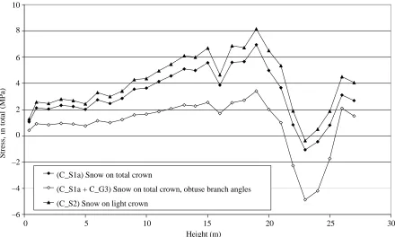
Snow load: The simulations of snow loads are based on an assumed snow accretion of 50 kg/m2_{, which should} cause a considerable stress, but not exceed the stability of the tree. With an estimation of about 15 m2 _{for the} hor-izontal crown projection, a snow mass of 750 kg, in total, be accumulated on the crown. C_S1a: Assuming that the branches carry snow masses proportional to the branch masses, and with 220 kg of branch fresh mass, in total, each branch shall support an additional snow mass 3.4 times its branch mass. The point of application of the snow-based gravity force is always mid-branch. In

C_S1b, this point is shifted outwards, to a distance of two-thirds of the branch length. In C_S2, with respect to the real shape of the crown, it is assumed that only the

branches of the light crown, above a height of 20.4 m, are covered by snow. The lower branches, reduced in length by shadowing, shall not carry an amount of snow worth mentioning. Given the same horizontal crown projection area, each branch of the light crown now supports a snow mass 4.4 times its own weight, as the fresh mass of these branches is 170 kg.

Aerodynamic properties: As aerodynamic properties of tree crowns show great variation and depend on the wind speed, C_P1 accounts for a modified function of the drag coefficient c_D. Based on experimental data (WALSHE, FRASER 1963; MAYHEAD 1973), a parabolic decrease is described, beginning with 0.7 at calm and end-ing with 0.22 at a wind speed v of 33 m/s. The fitted poly-nomial is c_D = 0.7093 – 0.0283v + 0.0004v2_{. In variant C_P2,} streamlining is expressed by the reduction of the sail area instead of a decreasing drag coefficient. On the assump-tion that the sail area is reduced by 20% at a wind speed of 10 m/s and by 60% at 20 m/s (PELTOLA, KELLOMÄKI

1993), the parabolic interpolation f_red= 1 – 0.01v – 0.001v2 is the reduction function which is valid in the range from 0 to 20 m/s. The drag coefficient is fixed at 0.35.

WIND CHARACTERISTICS AND WIND FORCES

Wind forces acting on the 17 differentiated crown sec-tions are derived from hypothetical wind condisec-tions for a north-western storm. In the absence of measured wind profiles within the stand, the potential function

v(z) = v_r⋅ (z/z_r)c ₍₃₎

is applied, which estimates the wind speed v at any height

z. It is v_r the given wind speed of 20 m/s at the reference height z_r, the height of the canopy, with z_r = 30 m. The exponent c is assumed to be 0.3 for forests (HÄCKEL 1993). (3) be valid for the wind conditions at stand edge. Dy-namic effects of gustiness or tree swaying are not consid-ered, wind speed is held constant and the tree shall deflect to a point of no return under wind loading. The wind force

F_W(z) acting on a sail area A(z) of a crown section at height z is given by

F_W(z) = 0.5 ⋅ρa ⋅cD⋅A(z) ⋅v2 (z) (4)

The air density ρa is assumed to be a constant with

1.2 kg/m3_{. The calculated wind forces shall be static and} act horizontally and directly on the mid-sections of the stem; there is no force transmission from branch into stem and therefore, possible torsional moments due to asym-metries of the crown are neglected.

Applying a static wind loading, due to a mean wind speed averaged over a certain time period, neglects the gustiness of the wind. This can lead to a considerable underestimation of experienced forces because the short-time maximum wind speed can be three short-times the mean wind speed.

de-fined as the ratio of the maximum bending moment to the mean bending moment (GARDINER et al. 1997, 2000):

G = BM_max/BM_mean with

BM_mean = (0.68s/h – 0.0385) + ( –0.68s/h + 0.4785) ⋅ (1.7239s/h + 0.0316)x/h

BM_max =(2.7193s/h – 0.061) + (–1.273s/h + 0.9701) ⋅ (1.1127s/h + 0.0311)x/h ₍₅₎

where 0.075 < s/h < 0.45 and with s (m) the mean spacing between the trees, h (m) the mean tree height and x (m) the distance from the forest edge. Concerning the Douglas fir stand, the average tree distance was estimated to be about 8 m, resulting in s/h≈ 0.25 and thus, at stand edge, in a gust factor of about 2.9. Gust factor estimations that are valid inside the stand require a further multiplier given by

f_stand = BM_mean (x)/BM_mean (x = 0). With respect to the position of the analysed tree, a distance of x = 50 m is chosen, giving a reduced within-stand gust factor of about 1.7.

Alternatively, instead of applying a gust factor, the mean wind speed can directly be set equal to the maxi-mum gusting wind speed, because it was shown that the extent of tree bending by gust maxima differs little from the degree of bending caused by a static wind of equal velocity (PELTOLA et al. 1993). This procedure is to be preferred in the case of simulating very high mean wind speeds as otherwise, an additional gust factor would re-sult in unrealistic high stress values.

Simulation variants

W_Ref refers to the potential wind profile of a north-western wind with a velocity of 20 m/s at canopy height (described above).

Wind velocity: In W_9, the velocity is 9 m/s. This vari-ant is chosen in combination with snow load simulations, because this wind speed is a limit above which snow can be dislodged from the branches (PELTOLA et al. 1997).

W_0 accounts for calm.

Wind profiles: W_P1 represents the logarithmic wind profile that is commonly used in wind models (e. g., PEL

-TOLA, KELLOMÄKI 1993; GARDINER et al. 2000). The ve-locity v(z) at height z is estimated by

v(z) = v_r [ln((z – d) /z₀ )/ln((z_r – d) / z₀)] (6) where v_r = 20m/sis the reference wind speed at height

z_r = 30 m. Taken from literature (GARDINER et al. 2000) are the values for the roughness length z₀ (m) and the zero plane displacement d (m). As a function of stand height

z₀ = 0.06 · h, the roughness parameter here is 1.8 m. Out-side the stand, the zero plane displacement can normally be neglected (PELTOLA, KELLOMÄKI 1993) and thus,

d = 0.

W_P2 describes an empirical, within-stand wind profile

v(z) = v_r · [1 + α(1 – z / z_r)]–2 ₍₇₎ proposed by LANDSBERG and JAMES (1971) for a Sitka spruce stand. The parameter α is extremely influenced by

the leaf-area density. But in the absence of such data, e. g., the refined approach of LANDSBERG and JARVIS

(1973) which accounts for this dependency could not be applied and thus, the constancy α = 2.5, proposed in the first-mentioned publication, was applied.

MODELLING ELASTOMECHANICS OF THE TREE

The central key for prognosticating stress and strain of the wood fibres in the stem for a given loading case is the calculation of the elastic curve of the stem axis. It is only the stable state of the bent tree, at standstill, which is of interest, when acting external forces and bending mo-ments are in equilibrium with counteracting internal ones. External bending moments result from wind forces and from gravity of tree masses (stem, branch, needle and possibly snow and ice masses) that are not symmetrical relative to a perpendicular axis going through the foot of the tree. The internal bending moments depend on area and form of the stem cross sections, the elastic properties of the wood and the degree of the curvature of the tree. With the differential equation system set up, finding the steady state will require an iterative solution, because any displacement of the tree and its masses will change the acting forces which, again, influence the displace-ment themselves.

Common basic assumptions and their adoption in the model

Usually, according to the theory of classic elastome-chanics, the stem of a tree is considered to behave as a beam (TIMOSHENKO 2000; SZABÓ 2001). It is to be prov-en whether the underlying assumptions in such a case actually hold true.

(i) If the ratio of length to diameter of a beam is great (> 20 : BAUMANN 1922; > 25 : SZABÓ 2001) transverse forces (shear) can be neglected. An initially even cross section will remain even and perpendicular to the bent stem axis.

For most trees, due to their slenderness, this is valid. Therefore, the strain of the fibres is proportional to the distance from the neutral axis. The neutral axis, related to a distinct cross section, is defined by the line of zero strain.

54 J. FOR. SCI., 48, 2002 (2): 49–69

(iii) The unloaded beam is not curved; its straight axis is given by the line which intersects the mass centroids of all cross sections. All external forces act perpendic-ularly on the axis of the stem and lie within a vertical plane, the force or momentum plane, which includes the tree axis.

In approximation, without loading of the tree, the axis of most stems may be straight, and therefore, this assump-tion is adapted here, too. But instead of mass centres, the centroids are derived by weighing with the bending stiff-ness of the year rings. As for the acting forces, due to non-homogeneous air flow and an asymmetric crown, normally they do not lie within a plane and moreover, do not run through the stem axis. Additional torsional mo-ments are the consequence.

In the present state of TREEFLEX, torsional moments are still ignored. But TREEFLEX has no restrictions con-cerning the acting force system and thus, as a full 3-D model, the spatial curvature of the axis can be represent-ed completely.

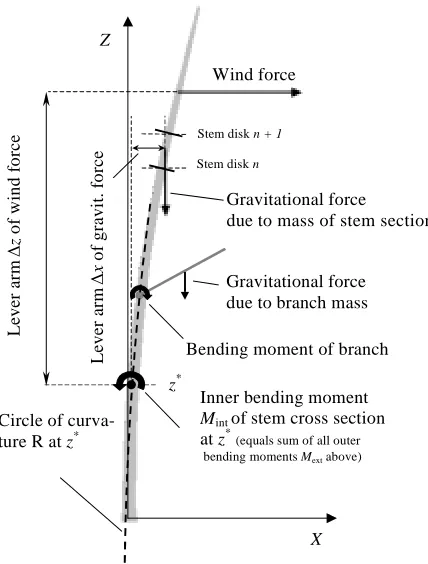
Stress and strain for a stem with irregular cross-sections and varying MOE

The stem of a tree is considered to be a perpendicular cantilever which is firmly clamped (stiff anchorage) at its foot, where the origin of a Cartesian co-ordinate system shall lie (Fig. 1). As stem analyses reveal, the form of the stem cross sections and of the inner year rings is rarely found to be circular or oval, but it can be extremely irreg-ular (Fig. 2). Furthermore, contrary to artificial materials, the mechanical properties of wood show no constancy

but vary spatially within a stem. In the model, it is as-sumed that each year ring differs in the MOE, but within a ring, the elasticity shall be constant. Thus, the wood of the stem is modelled as a composite (WAINWRIGHT et al. 1976; SPECK et al. 1990, 1996; VINCENT 1990) which con-sists of n layers with specific Young’s moduli E_i, i = l,...,n. (The vertical variation is also taken into account accord-ing to the disk-specific differences, but for simplification of the formulae, corresponding indices are omitted.)

In the case of an irregular shape of the cross section, the bending direction is of great importance. Referring to a distinct cross section (Fig. 2), a local co-ordinate sys-tem is chosen with the x-axis in bending direction and the origin in the neutral point, which is the Young’s-modulus weighted centre. Then, the y-axis coincides with the neu-tral axis a, and δ_a is the distance to a infinitesimal area dA_i

located in the i-th year ring, which has the area A_i. With respect to the location of the neutral axis, the axial second moment of area I_aof the total cross-sectional area A is the sum of all ring-specific contributions I_a,i.

2 ,

1 1 _i

n n

a a i i a

i i A

I I dA δ

= =

=

∑

∑∫

(Nm2_{) is the flexural stiffness (bending stiffness) which} characterises the resistance of the stem against bending (at a certain height). As the Young’s modulus E_i is ring-specific, the elasticity of the total cross section, denoted Z

X Wind force

Gravitational force due to mass of stem section

Gravitational force due to branch mass Bending moment of branch

Le

v

e

r

a

rm

∆

z

of

wi

nd

fo

rc

e

Le

v

e

r

a

rm

∆

x

of

gr

a

v

it

.

for

c

e

Inner bending moment Mintof stem cross section

at z*(equals sum of all outer

bending moments Mextabove)

z* Circle of curva-ture R at z*

Stem disk n Stem disk n + 1

Fig. 1. Acting forces and bending moments for a tree subjected to wind loads and self-weight

Fig. 2. Stem disk of Douglas fir No. 104 at a height of 0.40 m, considered to be a composite with ring-specific material proper-ties; location of neutral axis and neutral point according to given bending direction (year rings alternating in light and dark grey)

, st,

1

n a i

a i

i a

I

E E

I

=

=

∑

N

W E

S

Neutral axis a

Wind direction =: bending direction

Bark

Neutral point = the Young’s-modulus weighted centre

δa

dAi

i-th ring

Y

X

as the “structural” Young’s modulus E_st,a (SPECK et al. 1996), is given by

and thus, the flexural stiffness

, ,

1 1

n n

a i a i i i a i

At the state of equilibrium between the sum of all acting external bending moments and the counteracting inner ones, M_{ext, a} ≡M_{int, a}, the curvature 1/R of the stem axis (Fig. 1) is

As the stress σ_i(δ_a) in the i-th year ring at a distance δ_a from the neutral axis a is given by σ_i(δ_a) = E_i ·δ_a / R , and inserting (9) and (10), it is

Applying HOOKE’s law, the corresponding strain is

which illustrates that the strain in a specific year ring does not depend on its local, ring-specific elastic property but on the flexural stiffness of the total cross section. As usually maximum stress and strain at the periphery of the stem, experienced in the n-th year ring, are of interest, the maximum distance δmax, a to the neutral axis is to be

cho-sen.

A complete description of the differential equation ap-proach and its solution is given in the Appendix.

Technical details of modelling

At present state, the TREEFLEX simulation software consists of two, non-integrated modules. A conventional database stores measured geometry and material proper-ties data and calculates and exports, by Visual Basic® scripts, the complete data sets. These data are required by the second module (developed by the authors), which iteratively solves the differential equation problem for a given loading case. Output data are stress and strain at the stem surface and the displacement of the stem axis. Graphical visualisation with optional DXF and POVRay export is possible.

RESULTS

Each simulation of the elasto-mechanical bending of the tree is based on the characteristics, which are given in the chosen variant combinations for stem, crown and wind properties (Table 1). Calculated are the stress values at stem periphery (excluding bark) and at the heights of all stem disks. With respect to the wind direction, only data of the fibres oriented to north-west are presented because they experience the highest tensile stresses.

STRESS DISTRIBUTION OF THE REFERENCE VARIANT

The 3-D grid in Figure 3a, which presents the stress distribution at the stem surface, does not at all indicate ext,

st,

1 a

a a

M

R=E ⋅I (10)

(11) ext,

, 1

( ) i a a

i a n

i a i

i

E M E I

δ σ δ

=

⋅ ⋅

=

⋅

∑

(12) ext,

( )

( ) i a a a

i a

i a

M

E S

δ σ δ

ε δ = = ⋅

0.4 4 8

12 ₁₆

20 ₂₄ NW

E -20

-10 0 10 20

Stress (MPa)

Height (m) _Azimuth

Reference variant - surface stress distribution

Reference variant

Normalised stress and strain in NW fibres

0.4 0.6 0.8 1.0 1.2 1.4 1.6

0 5 10 15 20 25 30

Height (m)

Relative stress and strai

n _{Normalised stress}

Normalised strain

Fig. 3b. Normalised stress and strain for the reference variant (S_Ref + C_Ref + W_Ref) Fig. 3a. Surface stress distribution calculated for the reference

56

J. FOR. SCI.,

48

, 2002 (2): 49

–

69

Table 1. Results of the tree-bending simulations

Model variant combinations Height (m)

Stem Crown Wind 0.4 1.3 2.0 3.0 4.0 5.0 6.0 7.0 8.0 9.0 10.0 11.0 12.0 13.1 14.0 15.0 16.0 17.0 18.0 19.0 20.0 21.0 22.0 23.0 24.0 25.0 26.0 27.0

Tensile stresses in surface fibres oriented to NW (or NNW*) (MPa)

TREEFLEX

Reference variant

S_Ref C_Ref W_Ref 8.4 13.5 14.0 15.3 15.6 16.5 17.2 17.3 15.8 17.1 16.6 18.1 18.5 18.3 17.7 18.3 13.5 16.5 14.7 15.5 13.2 10.3 11.1 9.8 9.7 9.2 8.5 11.4 Stem geometry variants

S_G1 C_FEM W_Ref* 6.1 9.8 9.9 11.0 11.3 11.7 12.0 12.0 10.6 11.5 11.0 12.3 11.9 11.7 11.3 11.4 8.5 10.2 8.5 8.9 7.7 6.2 7.5 7.3 7.8 7.5 8.0 16.1 S_G2a C_Ref W_Ref 9.0 14.8 15.0 16.7 17.2 18.0 18.7 18.1 16.6 18.4 17.6 19.9 19.7 19.7 19.0 19.4 14.6 17.7 15.5 16.6 13.9 10.9 11.8 10.3 10.1 9.3 8.7 11.6 S_G2b C_Ref W_Ref 8.2 13.4 13.6 15.2 15.6 16.3 16.9 16.4 15.0 16.6 15.8 18.0 17.8 17.8 17.2 17.5 13.2 15.9 14.0 15.0 12.6 9.9 10.6 9.3 9.2 8.5 8.0 10.7 S_G3a C_Ref W_Ref 10.5 16.9 16.9 18.2 18.3 18.5 19.2 19.3 17.4 19.1 17.8 19.0 18.9 18.6 18.0 18.6 13.7 16.8 14.9 15.7 13.4 10.5 11.2 9.9 9.8 9.3 8.6 11.4 S_G3b C_Ref W_Ref 12.7 20.4 20.1 21.6 21.7 21.6 22.4 22.3 20.2 23.2 21.7 22.6 21.7 21.1 20.3 20.2 14.9 17.6 15.5 16.2 13.9 10.8 11.6 10.2 10.0 9.5 8.7 11.5 S_G3c C_Ref W_Ref 17.2 27.7 26.8 29.2 30.2 30.2 30.1 29.2 26.1 30.7 29.2 30.5 29.2 28.7 27.8 28.2 21.4 23.9 20.2 19.8 16.2 12.1 12.6 11.0 10.7 10.0 9.0 11.8 S_G3d C_Ref W_Ref 30.9 49.6 49.8 53.0 55.6 52.9 52.5 49.9 44.1 55.7 53.8 54.9 53.3 54.3 51.6 54.0 42.6 47.9 42.2 41.6 31.9 23.9 20.7 15.9 13.3 11.6 9.6 11.9 Stem wood property variants

S_WP1 C_Ref W_Ref 8.7 14.0 14.6 15.9 16.2 17.2 18.0 18.0 16.5 17.9 17.3 19.0 19.4 19.2 18.6 19.2 14.2 17.4 15.5 16.4 14.0 11.0 11.8 10.4 10.2 9.7 8.8 11.7 S_WP2 C_Ref W_Ref 8.2 13.2 13.7 15.0 15.3 16.3 16.9 16.9 15.5 16.7 16.2 17.7 18.1 18.0 17.4 17.9 13.2 16.3 14.5 15.2 13.0 10.1 10.8 9.6 9.5 9.1 8.6 11.5 S_WP3 C_Ref W_Ref 8.4 13.6 14.1 15.4 15.7 16.7 17.4 17.3 15.9 17.1 16.6 18.1 18.5 18.3 17.6 18.2 13.3 16.4 14.6 15.3 13.0 10.2 10.9 9.6 9.5 9.1 8.6 11.5 Crown geometry variants

S_Ref C_G1 W_Ref 7.0 11.2 11.6 12.7 12.9 13.7 14.3 14.3 13.1 14.2 13.8 15.1 15.4 15.3 14.8 15.3 11.3 13.9 12.4 13.1 11.2 8.8 9.3 8.2 8.1 7.7 7.1 8.7 S_Ref C_G2 W_Ref 8.7 14.1 14.6 16.0 16.4 17.4 18.2 18.3 16.8 18.3 17.7 19.5 20.1 20.1 19.6 20.5 15.2 19.0 17.2 18.6 16.2 13.0 13.7 12.1 11.1 9.6 8.7 11.6 S_Ref C_G3 W_Ref 8.5 13.6 14.1 15.4 15.7 16.6 17.3 17.3 15.8 17.1 16.6 18.1 18.4 18.2 17.6 18.1 13.3 16.3 14.4 15.1 12.9 9.9 10.9 9.9 9.9 9.4 8.7 11.1 Crown snow load variants

S_Ref C_S1a W _ 0 1.1 2.1 2.0 2.3 2.2 2.0 2.7 2.5 2.8 3.6 3.7 4.1 4.6 5.1 5.0 5.6 3.9 5.6 5.7 7.0 5.0 3.7 0.8 -1.1 -0.5 0.8 3.1 2.7 S_Ref C_S1a, C_G3 W _ 0 0.4 0.9 0.8 1.0 0.9 0.7 1.1 1.0 1.2 1.6 1.6 1.8 2.1 2.3 2.3 2.5 1.7 2.5 2.7 3.4 2.0 1.0 -2.3 -4.9 -4.2 -1.7 2.1 1.5 S_Ref C_S1a W _ 9 8.6 14.1 15.3 17.1 17.7 19.0 20.4 20.8 19.7 22.2 21.7 24.7 26.0 26.8 26.8 29.0 21.1 27.8 25.6 28.8 24.7 19.0 18.4 15.1 14.7 14.9 14.7 17.4 S_Ref C_S1b W _ 9 9.6 15.6 17.0 19.1 19.8 21.1 22.8 23.2 22.0 24.9 24.3 27.8 29.3 30.3 30.4 33.1 24.0 32.0 29.5 33.6 28.8 22.3 21.5 17.6 17.3 17.7 17.5 19.8 S_Ref C_S2 W _ 0 1.3 2.6 2.5 2.8 2.7 2.4 3.3 3.0 3.4 4.3 4.4 5.0 5.5 6.1 6.0 6.7 4.6 6.9 6.7 8.2 6.5 5.3 1.9 -0.4 0.5 1.9 4.5 4.1 Wind and crown aerodynamic property variants

S_Ref C_Ref W _ 9 2.5 4.0 4.2 4.6 4.7 5.0 5.2 5.2 4.8 5.2 5.0 5.5 5.7 5.6 5.5 5.7 4.2 5.2 4.7 5.1 4.3 3.3 3.1 2.4 2.5 2.7 2.9 3.8 S_Ref C_Ref W _ P 1 7.9 12.7 13.2 14.5 14.7 15.6 16.3 16.3 14.9 16.2 15.7 17.2 17.5 17.4 16.8 17.4 12.8 15.8 14.1 14.9 12.8 10.0 10.7 9.5 9.4 9.0 8.4 11.3 S_Ref C_P1 W_Ref 10.1 16.2 16.8 18.3 18.7 19.7 20.6 20.6 18.8 20.4 19.7 21.6 22.0 21.8 21.1 21.7 16.0 19.6 17.4 18.3 15.7 12.3 13.3 11.9 11.6 11.0 10.0 13.4 S_Ref C_P2 W _ P 1 5.2 8.3 8.6 9.5 9.6 10.2 10.7 10.7 9.8 10.6 10.2 11.2 11.5 11.4 11.0 11.4 8.4 10.3 9.2 9.7 8.2 6.4 6.6 5.6 5.5 5.4 5.3 6.9 S_Ref C_P1 W _ P 2 2.7 4.3 4.5 4.9 5.0 5.3 5.6 5.6 5.2 5.6 5.5 6.1 6.3 6.3 6.2 6.5 4.9 6.2 5.7 6.3 5.6 4.5 4.8 4.3 4.8 5.1 5.6 8.1

Finite element model

S_FEM C_FEM W_Ref* 4.5 10.1 8.0 10.2 10.6 10.4 11.6 11.5 8.9 10.6 9.9 12.0 10.3 12.6 10.8 11.3 8.0 10.2 7.9 8.8 7.9 5.9 7.9 7.9 8.5 8.5 9.5 25.3

0

5

10

15

20

25

30

0

5

10

15

20

25

30

Height (m)

Stress (MPa)

Finite element model

TREEFLEX

FEM variant vs. corresponding TREEFLEX variant Stress in NNW fibres

5

Stress (MPa)

0 10 15 20 25 30

30 25 20 15 10 5 0

Height (m) TREEFLEX

Finite elemet model

Fig. 4. Comparison between variants modelled with finite elements (S_FEM + C_FEM + W_Ref) and with TREEFLEX

(S_G1 + C_FEM + W_Ref), stresses presented for the outer fibres oriented to NNW

Cross section form variants vs. reference variant

-12% -9% -6% -3% 0% 3% 6% 9% 12%

0 5 10 15 20 25 30

Height (m)

% stress difference

Circular cross-sectional form Oval cross-sectional form

Cross section form variants vs. reference variant

% stress difference

Oval cross-sectional form Circular cross-sectional form

Height (m) 12

9 6 3 0 –3 – 6 – 9

15 –12

10 5

0 20 25 30

Fig. 5. Influence of the form of the stem cross section on experienced stresses, variants S_G2a (circular form) and S_G2b (oval form), combined with C_Ref + W_Ref

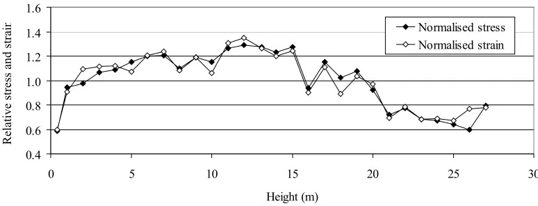
uniformity: regarding a fixed azimuth orientation, here NW, where stresses are maximum, the values are relatively small near the base of the stem (8 MPa), increase within the branch-free part of the bole (17–18 MPa), and decrease within the crown (8–9 MPa), but with a distinct rise in the uppermost part. Single major deviations, e. g., at the height of 16 m (13.5 MPa), find their explanation in local stem thickenings. The data rows of stress and strain can be best compared if they are normalised by the mean values (Fig. 3b). The curves are very similar; some distinct devi-ations are caused by a significant, locally increased or decreased wood density (mean density: 0.55 g/cm3_, maxi-mum density: 0.65 g/cm3 _{at 19 m, minimum density:} 0.44 g/cm3 _{at 26 m).}

FINITE ELEMENT MODEL VS. HOLISTIC APPROACH OF TREEFLEX

58 J. FOR. SCI., 48, 2002 (2): 49–69

Hollow stem variants - reduction in bending stiffness

0% 10% 20% 30% 40% 50% 60% 70% 80% 90% 100%

0 5 10 15 20 25 30

Height (m)

%

reduction

10 % rem. wall thickness at 1.3 m 20 % rem. wall thickness at 1.3 m 30 % rem. wall thickness at 1.3 m 40 % rem. wall thickness at 1.3 m

Hollow stem variants - stress increase compared to reference variant

0% 50% 100% 150% 200% 250% 300%

0 5 10 15 20 25 30

Height (m)

%

stress

increase

10 % rem. wall thickness at 1.3 m 20 % rem. wall thickness at 1.3 m 30 % rem. wall thickness at 1.3 m 40 % rem. wall thickness at 1.3 m

Height (m)

10% rem. wall thickness at 1.3 m 20% rem. wall thickness at 1.3 m 30% rem. wall thickness at 1.3 m 40% rem. wall thickness at 1.3 m

15 10

5

0 20 25 30

Height (m) Height (m)

15 10

5

0 20 25 30

Height (m) 100 80 60 40 20 % reduction 0

10% rem. wall thickness at 1.3 m 20% rem. wall thickness at 1.3 m 30% rem. wall thickness at 1.3 m 40% rem. wall thickness at 1.3 m

300 250 200 150 100 50 0

% stress increase

Fig. 6a. Hollow stem variants (S_G3a–S_G3d, combined with C_Ref + W_Ref) – reduction in diameter

Fig. 6b. Hollow stem variants (S_G3a–S_G3d, combined with C_Ref + W_Ref) – reduction in cross-sectional area Fig. 6c. Hollow stem variants (S_G3a–S_G3d, combined with C_Ref + W_Ref) – reduction in bending stiffness

Fig. 6d. Hollow stem variants (S_G3a–S_G3d, combined with C_Ref + W_Ref) – stress increase compared to reference variant

Hollow stem variants - reduction in diameter

0% 10% 20% 30% 40% 50% 60% 70% 80% 90% 100%

0 5 10 15 20 25 30

Height (m)

%

reduction

10 % rem. wall thickness at 1.3 m 20 % rem. wall thickness at 1.3 m 30 % rem. wall thickness at 1.3 m 40 % rem. wall thickness at 1.3 m

Hollow stem variants - reduction in cross-sectional area

0% 10% 20% 30% 40% 50% 60% 70% 80% 90% 100%

0 5 10 15 20 25 30

Height (m)

%

reduction

10 % rem. wall thickness at 1.3 m 20 % rem. wall thickness at 1.3 m 30 % rem. wall thickness at 1.3 m 40 % rem. wall thickness at 1.3 m

10% rem. wall thickness at 1.3 m 20% rem. wall thickness at 1.3 m 30% rem. wall thickness at 1.3 m 40% rem. wall thickness at 1.3 m

15 10

5

0 20 25 30

Height (m) 0 100 80 60 40 20 % reduction 15 10 5

0 20 25 30

Height (m) 100 80 60 40 20 % reduction 0

10% rem. wall thickness at 1.3 m 20% rem. wall thickness at 1.3 m 30% rem. wall thickness at 1.3 m 40% rem. wall thickness at 1.3 m

a – b –

c Hollow stem variants – reduction in bending stiffness d Hollow stem variants – stress increase compared to reference variant b Hollow stem variants – reduction in cross-sectional area a Hollow stem variants – reduction in diameter

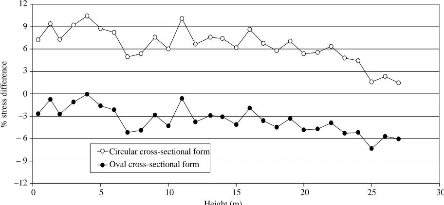
respondingly, oval cross sections modelled and oriented in order to approximately coincide with the form of the base disk result in equal or slightly reduced stresses at the stem base, but in increasing stress underestimation towards the top of the tree (–6%).

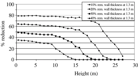
Of great importance is the simulation of partially rotten stems because it is often a decision of public safety whether such trees are to be removed, or not. Assuming a circular cross-section, a limitation of the supporting area to an outer ring, which has a remaining wall thickness of 40%, 30%, 20% or 10%, will result in an area reduction of 36%, 49%, 64% and 81%, and in a reduction in the axial second moment of area I (and bending stiffness S, too,if the area has a homogeneous MOE distribution) of 13%, 24%, 41% and 65.6%. These theoretical figures are ap-proximately verified (Fig. 6a–6c) when regarding the real cross sections and the calculated bending stiffness with respect to the neutral axis, i. e., here, with respect to the assumed south-eastern bending direction. It is found that these weakened stems will experience a stress increase of up to about 25%, 50%, 100% and over 250% at the stem base (Fig. 6d) if they do not break before, which is expect-ed to happen in the last case, because the absolute stress values of about 55 MPa exceeds the strength limit (Table 1).

EFFECT OF WOOD PROPERTIES

A general reduction of 20% of the wood density (and MOE) results in a stress increase from 4% (bottom) to 6% (mid-crown), and then, falling off, to 2% (top) (Fig. 7). The second-to-last year ring. Compared to the contour in

C_Ref, it is this “missing” last year ring which essentially contributes to the lack of bending stiffness of the very thin stem of the crown tip.

Fig. 4 shows the results of the finite element model and the holistic approach, i. e., the calculated stress values for the outer fibres oriented to north-northwest. Though, with the exception of the crown tip, the stress profiles match each other quite well, the (absolute) stress values of the finite element model are lower in the branchless part of the stem, with increasing divergence towards the foot and attain –15% (averaged for the lowest three heights). Probably, the deviation in modelling heart- and sapwood zones and thus, different gravity forces due to the inner mass distribution of the stem are, to some ex-tent, responsible. In contrast, at a height of 27 m, the fi-nite element model predict a more than 55% higher stress. This might be explained by the different way of how the models represent the last stem segment and the corre-sponding gravitational forces.

EFFECT OF STEM GEOMETRY

Cor-EFFECT OF CROWN PROPERTIES

A crown volume reduction of 50 % is accompanied by, on average, 18% decreased sail area (Figs. 8, 9, calculated by image analysis). As this variable directly affects the experi-enced wind forces, the stress reduction ranges between 15 and 24%. Less significant, if at all, is the effect of changing the branch angles, here, by substituting the original by ob-tuse ones. But very remarkable is the reaction of the highly asymmetric crown. The one-sided removing of branches re-sults mid-crown in a maximum stress increase of 25%.

EFFECT OF SNOW MASSES

If the masses of a snow fall of 50 kg/m2 _{are distributed} over the crown equally, i. e., each branch carrying a snow load proportional to its self-weight (variant C_S1a), then, already in calm, stresses up to 7 MPa are possible (Fig. 10a). The common centre of tree and snow masses lies outside the tree axis and is oriented to south-south-east. Thus, the stem is supposed to be bent in this direc-tion in the absence of wind. As stresses are calculated for the northwest and not for the north-northwest direction, these values do not represent the sustained maximum stresses which are (slightly) higher.

A peculiarity of this tree is a significant local crown mass eccentricity in the interval from 23 to 25 m due to missing southward-oriented branches. This causes a stress mini-mum, even with negative, i. e., compressive stresses at the north-west side of the stem. Unlike the case where wind forces dominate, at calm, obtuse branch angles significant-ly reduce stresses below a height of 20 m by 50 to 60%. Otherwise, the stress reversal in the mentioned asymmetric crown segment is enhanced because, in this variant, the branches stand away nearly horizontally (Fig. 8). Lastly, if

Fig. 8. Crown variants visualised with POV-Ray, view from NW. From left to right: reference, 50% volume reduction (C_G1), half-sided crown (C_G2) and obtuse branch angles (C_G3)

strain difference which follows an identical pattern is much higher because of the high deflection of the less rigid stem: it ranges from 25 to 29%. In contrast, in both other simulated wood-property variants, the magnitude of stress and strain differences are quite similar. A constant moisture content of 100% which slightly increases the stem mass in total effects relatively little, especially in the lower half of the stem. There are maximum changes be-tween + 1% and –2% . In the case of a uniform horizontal density and MOE distribution, the stresses decrease by 2%, with the exception of the uppermost stem part, where a minimal increase can be found.

Wood property variants vs. reference variant

-8% -6% -4% -2% 0% 2% 4% 6% 8%

0 5 10 15 20 25 30

Height (m)

%

stress

difference

14% 18% 22% 26% 30%

%

strain

difference

(S_WP2) Constant horizontal wood density

(S_WP3) Uniform moisture content of 100 %

(S_WP1) Wood density reduced by 20 %

(S_WP1) -''- but strain difference (right scaling)

Wood property variants vs. reference variant

(S_WP2) Constant horizontal wood density (S_WP3) Uniform moisture content of 100% (S_WP1) Wood density reduced by 20%

(S_WP1) –´´– but strain difference (right scaling)

% stress difference % strain difference

8 6 4 2 0 –2 –4 –6 –8

30

26

22

18

14 30 25

20

0 5 10 15

Height (m)

60 J. FOR. SCI., 48, 2002 (2): 49–69

the snow settles down only on the light crown, stresses in the main part of the stem are increased by 20%.

If wind is brought into play, at a wind speed of 9 m/s the contribution of the experienced stresses explained by the snow masses is between 70 and 80% (Fig. 10b), and total stress values of nearly 30 MPa are possible. Shifting the assumed snow mass centroids from mid-branch outwards (C_S2) enforces the stress by 11 to 19%.

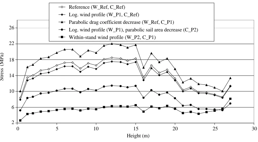
EFFECT OF WIND PROFILES AND AERODYNAMIC CROWN PROPERTIES

Relatively little changes, when instead of the potential wind profile (W_Ref) a logarithmic one (W_P1) is applied (Fig. 11a): the slightly reduced wind speed coincides with a stress difference of about 5% in the lower part of the stem. Much more influence is exerted by modifications of

Crown variants vs. reference variant

-30% -20% -10% 0% 10% 20% 30%

0 5 10 15 20 25 30

Height (m)

%

stress

reduction

(C_G1) 50 % crown volume

(C_G2) Half-sided crown

(C_G3) Obtuse branch angles

Crown variants vs. reference variant

(C_G1) 50% crown volume (C_G2) Half-sided crown (C_G3) Obtuse branch angles 30

20

10

0

–10

–20

–30

% stress reduction

15 10

5

0 20 25 30

Height (m)

Fig. 9. Influence of crown geometry on experienced stresses, variants C_G1, C_G2 and C_G3 compared to C_Ref, combined with S_Ref + W_Ref

Snow load variants - without wind

-6 -4 -2 0 2 4 6 8 10

0 5 10 15 20 25 30

Height (m)

Stress,

in

total

(MPa)

(C_S1a) Snow on total crown

(C_S1a + C_G3) Snow on total crown, obtuse branch angles

(C_S2) Snow on light crown

Snow load variants – without wind 10

8

6

4

2

0

–2

–4

–6

10 5

0 15 20 25

Height (m)

30

Stress, in total (MPa)

(C_S1a) Snow on total crown

(C_S1a + C_G3) Snow on total crown, obtuse branch angles (C_S2) Snow on light crown

the drag coefficient (C_P1) or of the streamlined sailing area (C_P2). The same magnitude of increase (about 20%) and decrease (about 40%) respectively, of these parame-ters, on average, is reflected in the change of stresses along the stem. In contrast, applying a quite different with-in-stand wind profile (W_P2) results in a diverging stress

pattern. Besides remarkably reduced stresses of 67% on average because of the lower wind velocity inside the stand, the normalised stresses are higher in the crown section; namely the uppermost values are striking (Fig. 11b).

Snow load variant - wind at 9 m/s

0 5 10 15 20 25 30 35 40 45

0 5 10 15 20 25 30

Height (m)

Stress,

in

total

(MPa)

(C_S1a) Snow mass centroid at 50 % branch length (C_S1b) Snow mass centroid at 66 % branch length Reference - no snow masses

Snow load variant – wind at 9 m/s (C_S1a) Snow mass centroid at 50% branch length

(C_S1b) Snow mass centroid at 66% branch length Reference – no snow masses

45

15 40

35 30 25 20 15 10 5 0

10 5

0 20 25

Height (m)

30

Stress, in total (MPa)

Fig. 10b. Effect of snow masses and their distribution (C_S1a, C_S1b), with wind (W_9), combined with stem properties of the reference (S_Ref)

Wind profile and aerodynamic crown property variants

2 6 10 14 18 22 26

0 5 10 15 20 25 30

Height (m)

Stress

(MPa)

Reference (W_Ref, C_Ref) Log. wind profile (W_P1, C_Ref)

Parabolic drag coefficient decrease (W_Ref, C_P1)

Log. wind profile (W_P1), parabolic sail area decrease (C_P2) Within-stand wind profile (W_P2, C_P1)

Reference (W_Ref, C_Ref) Log. wind profile (W_P1, C_Ref)

Parabolic drag coefficient decrease (W_Ref, C_P1)

Log. wind profile (W_P1), parabolic sail area decrease (C_P2) Within-stand wind profile (W_P2, C_P1)

Wind profile and aerodynamic crown property variants

Height (m) 26

15

Stress (MPa)

22

18 14 10 6 2

0 5 10 20 25 30

62 J. FOR. SCI., 48, 2002 (2): 49–69

SAFETY AGAINST FRACTURE FAILURE

Inverse to the stress and strain curves (Fig. 3a,b) are the curves which demonstrate the relative safety against fracture failure (Fig. 12). Safety is defined as the ratio be-tween breaking strength (modulus of rupture, MOR) and sustained stress or between strain at the proportional lim-it, where irreversible plastic deformation begins, and the

sustained strain. As the focus is on the living tree, the strength of the fresh wood of the stem is of interest. Un-fortunately, such measurements are rarely performed on complete, green stems (FONS, PONG 1957) but mostly on ideal specimen of green wood (U.S.D.A. Forest Products Laboratory 1989; WESSOLLY, ERB 1998). Therefore, to ac-count for the weakening influence of structural inhomo-geneities in the stem, the bending strength of the total

Wind profiles and aerodynamic crown properties

0,5 1,0 1,5 2,0 2,5 3,0 3,5

0 5 10 15 20 25 30

Height (m)

Normalised

stress

Reference (W_Ref, C_Ref)

Parabolic drag coefficient decrease (W_Ref, C_P1)

Log. wind profile (W_P1), parabolic sail area decrease (C_P2)

Within-stand wind profile (W_P2, C_P1)

Reference (W_Ref, C_Ref)

Parabolic drag coefficient decrease (W_Ref, C_P1)

Log. wind profile (W_P1), parabolic sail area decrease (C_P2) Within-stand wind profile (W_P2, C_P1)

Wind profiles and aerodynamic crown properties

Normalised stress

3.5

25 3.0

2.5

2.0

1.5

1.0

0.5

30 20

15 10

5 0

Height (m)

Fig. 11b. Effect of wind profiles and aerodynamic crown properties: normalised stresses by values at height 0.4

Reference variant - safety factors for stem breakage defined by stress and strain limits

1 2 3 4 5 6

0 5 10 15 20 25 30

Height (m)

Safety

factor

Local MOR = 38 - 56 MPa (red. factor = 0.85) Uniform MOR = 48.1 MPa (red. factor = 0.85) Strain limit = 0.004

Local MOR = 31 - 46 MPa (red. factor = 0.7) Uniform MOR = 23 MPa

Strain limit = 0.002

6

Reference variant – safety factors for stem breakage defined by stress and strain limits Local MOR = 38–56 MPa (red. factor = 0.85) Uniform MOR = 48.1 MPa (red. factor = 0.85) Strain limit = 0.004

Local MOR = 31–46 MPa (red. factor = 0.7) Uniform MOR = 23 MPa

Strain limit = 0.002 4

5

3

2

1

Height (m)

Safety factor

0 5 10 15 20 25 30

stem is reduced by 30% (FONS, PONG 1957; PETTY, WOR

-RELL 1981; PELTOLA, KELLOMÄKI 1993) or by 15% (PEL

-TOLA et al. 1999).

Referring to the breaking strength, for the investigated Douglas fir tree, a mean literature value of 48 MPa for green wood (with ρ₀ = 0.47g/cm3_{) was chosen (KOLL}

-MANN 1951). Reduced by a factor of 0.85 and corrected by the locally measured wood densities (in the range from ρ₀ = 0.44 g/cm3 _{to 0.65 g/cm}3_{), the estimated breaking} strength varies between 38 and 56 MPa. A reduction fac-tor of 0.7 results correspondingly in values from 31 to 46 MPa. If, simplified, an average density of the stem (0.55 g/cm3_{) is regarded, then the strength limit is uniform} 48 MPa (reduction factor of 0.85). In a further variant, a very low, uniform limit of 23 MPa is chosen according to WESSOLLY and ERB (1998). (The value of 20 MB, pro-posed by the authors, was adjusted due to the assumed higher MOE of the tree.)

In comparison to strength data, values for strain paral-lel to grain at the proportional limit for green wood are seldom published. For Douglas fir, WESSOLLY and ERB

(1998) state a strain proportional limit of 0.002, measured in compression. According to the U.S.D.A Forest Prod-ucts Laboratory (1989), values for compression perpen-dicular to grain range from 0.0024 to 0.0029 for green wood and from 0.0041 to 0.005 for wood at a moisture content of 12%. YLINEN (1942, 1952) published a value of 0.004 for compression parallel to grain (Scots pine, dry sample).

Thus, according to differently chosen strength and strain limits and reduction factors, the remaining minimum safety factor, which is always located mid-stem at a height of uni-form 12 m, varies from 1.2 (referring to the limit strength given by WESSOLLY and ERB [1998]) to 2.0 (reduction fac-tor 0.7) or 2.6 (reduction facfac-tor 0.85) (Fig. 12).

DISCUSSION

Model validation: When drawing conclusions from the above-given simulations, it must always be born in mind that the outcome of the model could not be verified by data measured on a real, elastically reacting tree. There-fore, at least, it was desirable to compare the results of two quite different models, the finite element model (GAF

-FREY et al. 2001) and TREEFLEX, the holistic approach, by checking corresponding stress prognoses for incon-sistencies, which could reflect principal model bugs. In this way, some errors (in both models) were found and removed. Remaining differences (Fig. 4) could not be at-tributed to any further possible errors, because not com-pletely met was the necessary precondition of absolutely equal modelling in both geometry and material properties of tree and acting forces. Especially model divergences of the uppermost stem part could account for the observed stress differences, because the thinner the stem the great-er will be the influence of changes in the cross-sectional form and absolute area of the stem, and of the forces. Thus, as prognosticated stress values cannot claim full validity, more importance is to be attached to their

magni-tude and the pattern of their distribution. In this sense, comparing both model approaches, it turns out that both trends for the vertical stress distribution coincide fairly well, which justifies the interpretation of the simulation results. Nevertheless, for a satisfying model verification, simulta-neously measured data of wind and fibre strain (BLACK

-BURN 1997; BLACKBURN, GARDINER 1997) remain desirable. The convergence of discretising and solving the dif-ferential equation system was successfully proven ex-emplarily. For the reference variant, the increase of sup-porting points from 9 to 17, to 33, and to 65 results in a change of the stem deflection (in, e. g., x-direction) of 6.6 cm, 1.0 cm and 0.3 cm maximum, respectively. The value of 6.6 cm found at 27 m is very little compared to the total deflection of 246 cm at that height. The numer-ical solution of the discretised equation system, using a Newton method, failed only in one case when a very high snow load on the light crown was combined with a high wind speed, resulting in an extreme deflection. (This simulation variant was, therefore, omitted.)

Hollow stems: Among all variants concerned with stem properties, the inner decomposition of a stem has the greatest effect on the stability of a tree. In the case of failure, in forest stands, this defect means economical loss but, e. g., in municipal locations, the endangering of pub-lic safety is the predominant aspect. As protection and preservation of old and big trees, which are often predes-tined to be hollow, is another declared public aim, experts are confronted with the dilemma deciding whether to fell or not to fell risk trees.

A simple, practical guideline is to spare those trees from felling which have a ratio of a remaining wall thickness to cross-section radius of more than 0.3 (MATTHECK et al. 1993; MATTHECK, BRELOER 1994). According to exten-sive surveys, such trees normally show sufficient resis-tance even in the heaviest storms. On the other hand, such a rigidly defined limit can imply the unnecessary removal of a high number of stable trees, too (SINN 1993; WESSOLLY 1993, 1995; WESSOLLY, ERB 1998), because trees with ratios of 0.1, or even less, can survive in storms. However, the stability of a tree must be analysed in com-bination with the state of the crown, which is mainly re-sponsible for the received wind forces. It is argued that the bending resistance of a hollow stem with a wall/radius ratio of 0.3 is reduced only by about 25% (WESSOLLY

1995), but it must be emphasised that the per cent stress increase will be, as shown for the investigated Douglas fir, two times higher (Fig. 6d). Further reducing the sup-porting wall causes an exponential stress increase (MAT

64 J. FOR. SCI., 48, 2002 (2): 49–69

(+160%) would be expected. Responsible is the horizon-tal shift of stem and crown masses and thus, the prolon-gation of the lever arms of the gravitational forces (Fig. 1): e. g., compared to the reference variant, the deflection of the stem in the south-east direction at a height of 27 m increases from 3.7 m to 10.3 m.

Lastly, it shall be mentioned that conventional calculat-ing of the mechanical stability is justified in the case of hollow stems, too (SPATZ et al. 1990; SPATZ 1994). Hollow stems with a wall thickness to a radius ratio greater than 0.1 do not show a significant ovalisation of the cross sec-tion and thus, the reducsec-tion of the axial second moment of area need not be taken into account.

Further stem properties: Compared to hollowness, the influence of other geometry or material properties of the stem extremely falls off, though it cannot always be ne-glected. For example, the ability to form reaction wood under constant (wind) forces results in oval stem cross sections which have, with respect to the wind direction, a higher axial second moment of area than a circular cross section equal in area. The gained stress reduction, of up to 10%, as shown in Fig. 5, would probably be greater, if the formed compression wood, its distribution and its mechanical properties, could have been taken into ac-count in the model.

A uniform horizontal distribution of the moisture con-tent, as well as of the wood density, affect little if the chosen values do not differ too much from the averaged ones, which are derived by the non-uniform distribution models. The differences in stem mass, in mass distribu-tion and in MOE distribudistribu-tion will alter the stresses only to a minor extent. Therefore, the application of such consi-derably simplified models seems legitimate. Greater devi-ations, e. g., the simulated 20% underestimation of wood density and MOE, cause increased stresses and especial-ly much higher strains because the softer material deflects much more under a given load. For this reason, as the stem wood of many trees or tree species show a signifi-cant vertical change in density (and MOE) (spruce, pine, birch: YLINEN 1952; spruce: BRÜCHERT et al. 2000; Cryp-tomeria japonica: KATO, NAKATANI 2000), this variation should be assessed – even in the case of tree species, as Douglas fir, which normally do not show such a trend, because the density variation between neighbouring stem sections can be very great (GAFFREY, SLOBODA 2001).

Crown properties and wind forces: The wind forces acting on the crown depend on several factors: the wind velocity and the wind profile, on the one hand, and the sail area and the drag coefficient of the crown, on the other. As the pattern of wind profiles in a stand is very individual and can reliably be defined only by measure-ments (AMTMANN 1986), in most simulations, trees are assumed to stand solitary in order to allow the applica-tion of theoretical profiles (PELTOLA et al. 1999; GARDI

-NER et al. 2000; SPATZ, BRÜCHERT 2000), such as the potential or the commonly preferred logarithmic profile. If their parameters are correspondingly chosen for a given case, the derived absolute and, in particular, relative stress

distributions on the surface of the stem differ little in com-parison to the one which is induced by a (hypothetical) within-stand wind profile (Fig. 11b). This demonstrates the importance of knowing in detail the acting wind forces, if, e. g., for a tree in a stand, the phenomenon of adaptive growth, i. e., the relationship between experi-enced stresses or strains and growth in diameter, shall be studied (GAFFREY, SLOBODA 2001).

The wind load on a crown is proportional to its sail area and to its drag coefficient. But the problem is the stream-lining effect: both factors are reduced with increasing wind speed. To allow simplified modelling, either the sail area is held constant (WALSHE, FRASER 1963; MAYHEAD 1973) and the drag coefficient is variable, or vice versa (PELTO

-LA, KELLOMÄKI 1993). Unfortunately, applying both methods with the proposed parameters does not at all lead to congruent results (Fig. 11a). Indeed, it is hardly realisable or even impossible to accurately determine a function for the sail area or the drag coefficient reduc-tion for an individual tree. Applying literature data will always remain very uncertain in view of the highly differ-ing tree-specific crown properties.

Distribution of masses and gravitational forces:

Though the mass of the stem is usually several times the mass of the crown (in the case of the studied tree: 920 kg vs. 220 kg), gravity forces of the latter contribute in great-er part to the acting bending moments, at least in the up-per half of the stem (PELTOLA, KELLOMÄKI 1993), because these masses, which are never symmetrically dis-tributed with respect to the axis of the stem, are located more outward. If trees are leaning instead of standing upright, stresses can considerably be increased, too (SPATZ, BRÜCHERT 2000). In the above given example of the one-sided damaged, asymmetric crown (Fig. 9) stress-es can locally be higher by 25%. Lastly, the effect of the localisation of masses on bending stresses is demonstrat-ed by shifting the centroids of snow masses from mid-branch to a more peripheral position (Fig. 10b).

It was supposed that the angles of the main branches have great influence on the stability of the tree: the mass-es of branchmass-es that hang downward should rmass-esult in re-storing bending moments, which counteract the bending of the tree (MÖHRING 1980, 1981). This could not be con-firmed; the modification of the branch angles shows near-ly no effect (Fig. 9). As very high wind forces were acting in this simulation, the effect of the crown-mass related gravity forces might be secondary and masked. However, in the absence of wind and if a heavy snow load (750 kg) covers the crown, the tree with obtuse branch angles is indeed remarkably more stable: stresses are reduced by 50% and more (Fig. 10a).

Safety against fracture: Here, safety is considered only as stability against snapping of the stem and not as sta-bility against tree overturning, which might be less (PEL

the calculated safety factors underestimate the true safe-ty reserve.

In the variants presented in Fig. 12, at first view, striking are the enormous differences in calculated minimum safe-ty factors, which range from a critical value of 1.2 to a quite sufficient one of 2.6. But this must be seen in perspective with the purpose of defining the strength lim-its that are applied in the variants. The reference value of 48 MPa for maximum breaking stress in bending, the re-duction factors of 0.7 or 0.85, and the proportional strain limit of 0.004 are given just as they are expected to repre-sent the limit of fibre crushing. In contrast, the values of WESSOLLY and ERB (1998) contain a “safety supplement” because these published data are used by publicly ap-pointed tree experts who have to evaluate the risk that emanates from a tree. The safety supplement shall avoid or, at least, minimise incorrect decisions that trees, which are expected to be safe, fail and cause damage, which could give rise to possible recourses. Moreover, in prac-tise, taking wood samples to determine mechanical prop-erties is normally too expensive, if, at all, allowed because of injuring the tree. Alternatively, strength data are taken from literature and therefore, these should be the lowest values. In this sense, instead of the crushing strength in bending, the lower one in compression (20 MPa) was pub-lished (WESSOLLY, ERB 1998). Correspondingly, a strain limit of 0.002 was chosen, which indicates the beginning of plastic deformation under compression, but not the point of fibre breakage.

Regarding the question of whether breaking stress or strain at the proportional limit shall be used as a refer-ence, the advantage of the latter is its much lower varia-tion (YLINEN 1942; WESSOLLY 1995; WESSSOLLY, ERB

1998). Indeed, the variation of the wood density and thus, of the derived breaking strength is also high for Douglas fir (SLOBODA, GAFFREY 1999; GAFFREY, SLOBODA 2001). If this vertical variability of the MOE is taken into ac-count, the curve of the stress-based relative safety coin-cides very well with the one which is determined by the limit strain (Fig. 12, reduction factor 0.85). But, on the other hand, relating the estimated stresses to an average breaking strength instead of to locally calculated ones usually does not cause great differences but at single locations (e. g., at 17 m and 26 m). Therefore, the use of mean strength values as a reference seems to be justified, too.

The above made safety estimations only account for short-term loadings as it is the case for wind forces. If considerable snow masses remain on the crown for a longer time, the breaking strength is remarkably re-duced. As the wood structure will plastically deform (creeping) under long-term loading, the final break will take place at about 50% of the value under short-term loading (HALL 1967; WORRELL 1979; PETTY, WORRELL

1981). Regarding the snow-loaded Douglas fir tree in the absence of wind, the tree will still be far away from any risk of stem breakage (Fig. 10a). But as soon as a heavy wind blows, the stem is supposed to snap somewhere at

the height between 15 and 20 m (Fig. 10b). In combina-tion with wind, it is the gravity force of the snow masses that is mainly responsible for the bending stresses (70–80%), whereas the stress contribution of the wind is 10–20%, of the branch masses 5–7%, and of the stem mass only 0–2%. Comparable results are given by PEL

-TOLA et al. (1997).

As severe snow damage disasters occur more or less regularly, aspects of evaluating and improving the stabil-ity of single trees or entire stands under snow and wind loads have intensely been discussed (MÖHRING 1980; PETTY, WORRELL 1981; ROTTMANN 1985; MARSCH

1989; PELTOLA [ed.] 2000). Stem taper is the most impor-tant influencing characteristic: trees with a taper of 1:120, and still of 1:100, are considered to be very unstable (PEL

-TOLA et al. 1997). For example, for young spruce (data were derived from a 14-year old tree), the risk of stem failure, by calculating the Euler buckling load, is estimat-ed to be much higher (MARSCH 1989): already in the ab-sence of wind, snow masses of 50 kg/m2 _{can cause} buckling of stems with a taper of even 1:80 or 1:90. But it must be pointed out that for the young spruce trees, the assumed mass relations of branch mass to stem mass to snow mass are 1:2.2:9.3 (calculated by the averaged mass-es for the taper of 1:80 and of 1:90) whereas, e. g., for the 64-year old Douglas fir tree with a taper of 1:86, the rela-tions are 1:4:3.4. The much higher proportion of snow mass on the spruce crown will explain that buckling is already a risk at wind calm. Apart from the slenderness of the stem