Abstract — This paper presents a development of a design of experiment technique for quality improvement in automotive manufacturing industrial. The quality of interest is the colour shade, one of the key feature and exterior appearance for the vehicles. With low percentage of first time quality, the manufacturer has spent a lot of cost for repairing work as well as the longer production time. To permanently dissolve such problem, the precisely spraying condition should be optimised. Therefore, this work applied the multiple regression and response surface methods or RSM to investigate significant factors and to determine the optimum factor level in order to improve the quality of paint shop. Firstly, 2k full factorial was employed to study the effect of five factors including the paint flow rate at robot setting, the paint levelling agent, the paint pigment, the additive slow solvent, and non volatile solid at spraying of atomising spraying machine. The response value of colour shade at 15 and 45 degree are measured using spectrophotometer. Then the regression models of colour shade at both degrees were developed from the significant factors affecting each response. Consequently, both regression models were placed into the form of linear programming to maximise the colour shade subjected to 3 main factors including the pigment, the additive solvent and the paint flow rate. This led to the determination of new levels of decision variables and brought 70 % reduction on paint repairs cost and improve first time quality from 70% to 88% for the production of interest
Index Terms — Precisely Atomising Spraying Process, Colour Shade Mismatch, Multiple Regression, Constrained Response Surface Optimisation
I. INTRODUCTION
Currently, the stiff competition in automotive firm increases the need for quality improvement. The selections of the vehicle are based on the performance, the feature and the appearance. The first two are the perceived quality for each company. For the appearance, a colour shade, and paint durability are important since they are the first noticeable
Manuscript received December 29, 2009. This work was supported in part the Thailand Research Fund (TRF), the National Research Council of Thailand (NRCT), the Commission on Higher Education of Thailand and the Faculty of Engineering, Thammasat University, THAILAND.
* Y. Suwankham is with the Industrial Statistics and Operational Research Unit (ISO-RU), Department of Industrial Engineering, Faculty of Engineering, Thammasat University, 12120, THAILAND [Phone: (662)564-3002-9; Fax: (662)564-3017; e-mail: [email protected], [email protected]].
S. Homrossukon is an Assistant Professor, ISO-RU, Department of Industrial Engineering, Faculty of Engineering, Thammasat University, 12120, THAILAND.
P. Luangpaiboon is an Associate Professor, ISO-RU, Department of Industrial Engineering, Faculty of Engineering, Thammasat University, 12120, THAILAND.
quality for the user. It is found that the case of interest has faced with the problem of lower quality of colour shade at the final quality gate of assembly. The colour of body and the painted hang on the part are mismatch being complained by customer. The first time quality is low at 70%, especially for silver colour tone, resulting in high production cost for repairing and retrofitting. Furthermore, the production lead time is longer due to the change of a new painted part from supplier. To decrease such problem, a precisely atomising spraying bell gun, the new spraying technology is invested for car painting process. The selected machine would provide a good appearance, good levelling rate of spraying, good metallic effectand can also reduce consumption of purging and solvent being good for environment[1].
With high technology machine, the problem has still existed. It is found that the process performance capability (Ppk) is still quite low at 1.05 comparing to the minimum
target at 1.33, as shown in Fig 1. In this case, the deep detail of spraying process should be investigated so that the optimum working condition would be determined. Consequently, the problem of interest would be dissolved.
Fig.1 Performance of Current Operating Condition
II. PRECISELY ATOMISING SPRAYING PROCESS (PASP)
A. Process Review
Paint shop consists of four operation steps as shown in Fig 2. The electrodepositing film is performed in the first step. Joint and hem flange of bodies are sealed in the second step to prevent corrosion. The final process is inspection and polishing a painted body. These three processes do not relate to an exterior spraying, the third step, since they are separated and unrelated processes. In this case, the cause of the problem is narrowed to the process of spraying and coating. However, this study also waives the primer spraying and baking condition because there have been found commonly with other
Constrained Response Surface Optimisation for
Precisely Atomising Spraying Process
Y. Suwankham*, S. Homrossukon and P. Luangpaiboon
,Member, IAENG
1.0 0.8 0.6 0.4 0.2 -0.0
USL P rocess D ata
S ample N 100 S tD ev (O v erall) 0.205635
LS L *
Target * U S L 1 S ample M ean 0.3509
O v erall C apability
C pm * P p * P P L * P P U 1.05 P pk 1.05
O bserv ed P erformance P P M < LS L * P P M > U S L 10000.00 P P M T otal 10000.00
E xp. O v erall P erformance P P M < LS L * P P M > U S L 798.22 P P M Total 798.22
colour. Therefore, the determination of the base coating operation using atomising spraying robot, as shown in Fig 3 is mainly focused.
Fig.2 Details of PASP
Fig.3 Operation Process of Atomising Spraying Robot
B. Atomising Spraying Process
From Fig 3, paint was pumped from the mixing tank through the line to the paint booth. Gear pump help controlling paint flow rate while pressure air is supplied to atomising robot for driving bell dish to disperse the paint material into very small flaked size. Spraying will resume when the vehicle is transferred to the zone where robots R1 and R2 will perform the first coat on the exterior fender, the doors, the pillars, the box side, and the exterior tailgate panel surfaces. Robot R4 will paint the hood, the roof, and the box floor surfaces. Robots R3 and R6, then, perform the second coat for the area being first coated form R1 and R2 whereas the robot R5 will process the second coat for the rest. Once painting is completed, all robots will return to the original stage and prepare the color for the next vehicle. Painted body will be flashed before spraying clear coat and baking. Finally, the painted will be assessed based on the key product characteristics including film thickness, smoothness, glossy and color shade.
C. PASP Parameters
Control parameters of base coat include the paint material, spraying robot setting, the velocity of down draft air, booth temperature, and humidity. By brainstorming from the teams who work for a paint shop, e.g. product and process engineers, maintenance operators, quality engineers and paint suppliers it
has been found that the five key controllable parameters are declared including (1) a paint flow rate at robot setting, (2) a paint levelling agent, (3) a paint pigment, (4) a additive slow solvent, and (5) non volatile solid at spraying. Although there are many conditions for setting the robot, such as a gun distance, a bell speed, a shaping air, a voltage, but these conditions were fixed at the specific standard performance of the machine.
D. PASP’s Quality Measurement
The problem of interest is the mismatch of colour shade, especially for silver colour. Silver colour is bright shade and more sparkling from aluminium pigment; therefore, the brightness and the darkness were selected as the control value calling “L value”. It consists of the determination of colour shade at 15 and 45 visualised degrees.
III. METHODOLOGY FOR COLOUR SHADE MISMATCHED IMPROVEMENT
A. Response Surface Methodology (RSM)
The steepest ascent procedure, proposed by Box and Wilson [2], has been widely used in the area of Response Surface Methodology (RSM) or EVolutionary OPerations (EVOP). The objective of the RSM is to describe how the response of a process varies with changes in k process variables (Fig. 4). The process variables determined will depend on the specific field of the application [3].
Fig.4 Response Surface and its Contour Plot Most industrial processes have some process variables. For example, a response in a chemical reactor might be
concentration of product and the process variables affecting
this concentration might be temperature and pressure of a chemical plant [4]. The process variables such as speed of
lathe and advance of cutting tool in machining can be adjusted
by plant operators or by automatic control mechanisms to enhance the efficiency of the machine. Care must be taken to operate industrial processes within safe limits, but optimal conditions are rarely attained and increased international competition means that deviations from the optimum can have serious financial consequences. In many cases the optimum changes with time and there is a need for a routine mode of operation to ensure that the process always operates at optimal or near-optimal conditions.
On the theory and practice of RSM, it is assumed that the mean response (η) is related to values of the process variables (ξ1, ξ2, …, ξk) by an unknown function f. The functional
variables can be written as η = f(ξ), if ξ denotes a column vector with elements ξ1, ξ2, …, ξk. Estimation of such
surfaces, and hence identification of near optimal settings for process variables is an important practical issue with interesting theoretical aspects. The procedure begins with a factorial experiment around the prevailing operating condition. A sequence of first order models and line searches are justified on the basis that such a plane would be fitted well as a local approximation to the true response [5]. The estimated coefficients for the first order model are determined using the principles of least squares. A sequence of runs is carried out by moving in the direction of steepest ascent. When curvature is detected, another factorial experiment is conducted. This is used either to estimate the position of the optimum or to specify a new direction of steepest ascent.
In this study, response surface method is deployed to set up a relationship of the targeted and constrained responses and influential process variables. Sequential procedures of RSM are followed. A factorial experiment design is used to investigate the responses of the process. Analysis of variance (ANOVA) is then applied to find statistically significant process variables and determine the most effective levels. Regression analysis is used to fit a relationship equation of the response and its process variables. A restriction of process variables is also considered as the constraints of the process. A use of mathematical programming is to find the optimal levels in each process variables that can bring the suit levels of colour shade in both measurements of 15 and 45 degrees.
B. Constrained Response Surface Optimisation (CRSO)
In order to optimise the response of the brilliance of colour shade (L value) that might be influenced by several process variables, various sequential procedures via statistic tools are then used. One among those is the multiple regression analysis. It is used to determine the relationship between the influential variable of x’s and the dependent variable or response of y that is modelled as a linear or nonlinear model. Multiple regression fits a nonlinear relationship between the value of x’s and the corresponding conditional mean of y and has been used to describe nonlinear phenomena. Although Multiple regression fits a nonlinear model to the data, as a statistical estimation problem it is linear, in the sense that the regression model is linear in the unknown parameters which are estimated from the experimental data.
Multiple regression models are usually fit using the method of least squares. The least-squares method, published by Legendre and Gauss, minimises the variance of the unbiased estimators of the coefficients. Multiple regression analysis played an important role in the development of regression analysis, with a greater emphasis on issues of design and inference. The aim of regression analysis is to formulate a model of the expected value of a dependent variable y in terms of the value of an influential variable (or vector of influential variables) of x’s. In multiple linear regression, the model
0 1
k
i i i
y
β
β
x
ε
=
=
+
∑
+
is used, where ε is an unobserved random error with mean zero conditioned on a scalar influential variables of x’s. In this
model, for each unit increase in the value of x, the conditional expectation of y increases by units of . Conveniently, these models are all linear from the point of view of estimation, since the regression model is linear in terms of the unknown parameters of β0, β 1, .... Therefore, for least squares
analysis, the computational and inferential problems of multiple regressions can be completely addressed using the multiple regression techniques. This is done by treating
x, x2, ... as being distinct independent variables in a multiple
regression model.
The procedure of steepest ascent is that a hyper plane is fitted to the results from the initial 2k (fractional) factorial
designs. The direction of steepest ascent on the hyper plane is then determined by using principles of least squares and experimental designs. The next run is carried out at a point which is some fixed distance in this direction and further runs are carried out by continuing in this direction until no further increase in yield is noted. When the response first decreases another 2k design is carried out, centred on the preceding
design point. A new direction of steepest ascent is estimated from this latest experiment. Provided at least one of the coefficients of the hyper plane is statistically significantly different from zero, the search continues in this direction. More details are referred to in many statistical texts, for example [6] and [3]. Once the first order model is determined to be inadequate, the area of optimum is identified via a finishing strategy [7]. The procedure of steepest ascent method is shown in Fig. 5.
Many response surface problems involve the analysis of several responses or product specifications. However, they can be categorised in to the major and minor responses when compared. In this research, the main objective is to focus on the only one response of y1 and the remaining of y2 will turn to
be only the constraints that need to be met their acceptable ranges. The method of constrained response surface optimisation (CRSO) is then applied for this study. Either linear or non linear programming methods will be fitted to measure the most suitable to the problems. Moreover, the boundary limitations of the process variables are also determined as model constraints. The details of sequential procedure for setting up the optimum value via a relationship of significant variables and responses are followed.
1. Fit various multiple regression models associated with influential variables and its response of colour shade data at 15 degree measurement and formulate the most suit model as a problem objective.
2.Fit various multiple regression models associated with influential variables and its response of colour shade data at 45 degree measurement and formulate the most suit model as a problem constraint to meet its specification. 3. Complete the models above with the limitation of
feasible ranges of the process variables of x and form a
model as follow. Maximise ˆy1
Subject to x and ˆy2the requirement, where ˆy1 and ˆy2 are estimated major and minor responses, respectively.
5. Possibly adjust the obtained levels of process variables to implement the process of PASP.
[image:4.595.49.281.110.373.2]Fig.5 Flowchart of the Steepest Ascent Method to Improve the Process Response towards the Optimum [8]
IV. EXPERIMENTAL RESULTS AND ANALYSES
[image:4.595.330.523.355.613.2]From previous discussion, the response of colour shade difference or mismatch categorised are measured 15 and 45 degrees. The lower and upper specifications for both measurements are shown in Table 1. In the preliminary study, a two level experimental design was performed to determine the statistically significant from five process variables which consist of the pigment (A), levelling agent (B), additive solvent (C), percentage of paint solid (D) and paint flow rate of atomising spraying machine (E). The feasible ranges and the current operating condition is provided in Table 2.
Table 1 Process Responses and their Feasible Ranges Feasible Ranges Responses
[image:4.595.65.256.557.607.2]Lower Upper L15 -2.60 -0.30 L45 -0.50 +2.50
Table 2 Process Variables, their Feasible Ranges and Current Operating Conditions
Feasible Ranges Factors
Lower Upper Current A 6.14 6.40 6.40 B 0.92 1.51 1.00 C 0 3.2 1.50 D 70.1 76.8 74.6 E 180 250 250
At this step of using a factorial experiment design the objective is to analyse both main effects of process variables
and also its interaction effects. A 25 experimental design with
single replicate provides 32 treatments. The two levels of low and high are selected cover values of feasible ranges from the actual operating conditions in production line. Responses were measured and categorised by the different measurements of colour data at 15 and 45 degrees.
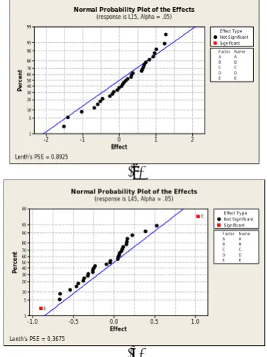
The primary goal of screening experimental designs is to investigate the critical few factors or process variables that influence the responses of colour data at 15 degree and 45 degree measurement. There are two graphs of Normal and Pareto plots, to be used to identify these influential factors. From the normal probability plot the relative magnitude of the effects are compared and evaluated their statistical significance. If design points do not fall near the line usually signal important effects, important effects are larger and further from the fitted line than less important effects. Less important effects seem to be smaller and centred around zero. In this preliminary study, it has been shown that with the normal probability plot using a significance level of 0.05, there is no significance effect on the response of colour data at 15 degree or no colour shade mismatch (Fig. 6(a)). In contrast to this, the main factors of C and E affect the response of colour data at 45 degree (Fig. 6(b)).
Effect
Pe
rc
e
n
t
2 1 0 -1 -2
99
95 90
80 70 60 50 40 30 20
10 5
1
F actor
D E E Name A A B B C C D
Effect Type Not Significant Significant
Normal Probability Plot of the Effects
(response is L15, Alpha = .05)
Lenth's PSE = 0.8925
(a)
Effect
Pe
rc
e
n
t
1.0 0.5 0.0 -0.5 -1.0
99
95 90
80 70 60 50 40 30 20
10 5
1
F actor
D E E N ame A A B B C C D
Effect Ty pe Not Significant Significant
E
C
Normal Probability Plot of the Effects
(response is L45, Alpha = .05)
Lenth's PSE = 0.3675
(b)
Fig.6 Normal Probability Plot of Effects for Responses of Colour Shade at 15 (a) and 45 (b) Degrees
The experiments were analysed using a general linear form of analysis of variance (ANOVA) including a source of variance and P-value as shown in Table 3. Numerical results with the terms in the model up through the third order reveal that significant variables (to L15) consist of A, C and E as the
[image:4.595.49.285.639.724.2]Table 3 ANOVA with all Main Effects and Estimable 2 and 3-Way Interactions for the 25 Full Factorial Designs with Single
Replicate
Sources of Variation
P-value for L15
P-value for L45
A 0.042 0.054
B 0.596 0.840
C 0.053 0.003
D 0.989 0.198
E 0.075 0.006
A*B 0.289 0.501
A*C 0.922 0.080
A*D 0.760 0.828
A*E 0.327 0.050
B*C 0.771 0.521 B*D 0.343 0.624 B*E 0.138 0.147 C*D 0.129 0.761 C*E 0.456 0.689 D*E 0.350 0.701
In order to determine the appropriate setting of the decision variables, the main and interaction effect plots on the experimental results based on each improvement operation were illustrated in Figures 7 and 8. When compared to the previous operating condition, proper levels of the decision variables on L15 from main effect plots are 6.14, 0, and 250 for A, C and E, respectively (Fig. 7). When focusing on L45, it has been shown that A, C, and E are set at 6.14, 0 and 250, respectively, from both main and interaction effects (Fig. 8). These results are summarised in Table 4.
Me
a
n
o
f L
1
5
6 .4 0 6 .1 4 -2 .0 -2 .4 -2 .8 -3 .2 -3 .6
3 .2 0 .0
2 5 0 1 8 0 -2 .0 -2 .4 -2 .8 -3 .2 -3 .6
A C
E
M a in Effe cts P lot (data mea ns ) for L 1 5
Fig.7 Significant Main Effect Plots for L15
Me
a
n
o
f L
4
5
6.40 6.14 1.50 1.25 1.00 0.75 0.50
3.2 0.0
250 180 1.50 1.25 1.00 0.75 0.50
A C
E
Main Effects Plot (data means) for L45
E
Me
a
n
250 180
2.00
1.75
1.50
1.25
1.00
0.75
0.50
A 6.14 6.40
Interaction Plot (data means) for L45
[image:5.595.301.554.199.385.2]Fig.8 Significant Main and Interaction Effect Plots for L45
Table 4 Summarised Main and Interaction Effect of Influential Variables from Preliminary Experiment
Influential Variables Responses
Main Effects Interaction Effects
L15 A, C, E None
L45 A, C, E AC, AE
The goal of the primary data analysis in Fig. 6 is to identify statistically significant variables and their interactions. Although some analytical results via normal probability plot of effect and analysis of variance are slightly different, the sequential procedures of the constrained response surface optimisation method (CRSO) consider all process variables affecting the responses following Table 5.
Table 5 A Comparisons of Influential Variable Levels after the First Improvements
Operating Conditions Parameters Decision Variables
Current 1st Cycle
A Pigment 6.40 6.10
B levelling Agent 1.00 0.50
C additive solvent 2.50 1.82
D Percentage of Paint Solid
74.6 74.6
E Paint Flow Rate of Atomising Spraying Machine
250 300
L15 Colour Data at 15
Degree of Measurement
-0.40 -1.37
L45 Colour Data at 45
Degree of Measurement
2.30 1.44
The method of steepest ascent is then applied to determine to the most preferable fitted equation of associated process variables to the responses of L15 (Fig. 9) and L45 (Fig. 10).
The regression equation is
L15 = 30.7 - 5.84 A - 0.440 C + 0.0181 E
Predictor Coef SE Coef T P-Value
Constant 30.660 14.630 2.100 0.045
A -5.837 2.313 -2.520 0.018
C -0.440 0.188 -2.340 0.027
E 0.018 0.009 2.100 0.045
Analysis of Variance
Source DF SS MS F P-Value
Regression 3 47.101 15.700 5.430 0.005
Residual Error 28 81.033 2.894 2.894
[image:5.595.51.287.447.666.2]Total 31 128.134
Fig.9 Regression Model on L15 including its significant coefficients and ANOVA Table
The regression equation is L45 = - 9.54 + 2.02 A + 0.323 C - 0.0129 E
Predictor Coef SE Coef T P-Value Constant -9.541 7.503 -1.27 0.214 A 2.019 1.187 1.7 0.1 C 0.32344 0.09641 3.35 0.002 E -0.01288 0.00441 -2.92 0.007
[image:5.595.305.550.455.536.2]Analysis of Variance Source DF SS MS F P-Value Regression 3 17.2728 5.7576 7.56 0.001 Residual Error 28 21.319 0.7614 0.7614 Total 31 38.5918
Fig.10 Regression Model on L45 including its significant coefficients and ANOVA Table
[image:5.595.302.551.588.668.2]CRSO, the response models where ˆy1 and ˆy2 can be linear, quadratic or even cubic polynomials. A nonlinear programming algorithm has to be used for the optimisation of a generalised reduced gradient algorithm to guarantee global optimal solutions.
The estimates of coefficients were significant from the table of testing individual regression of coefficients. The values of three components (A, C, E) of a PASP need to be selected to maximise a major response, Colour data at 15 (L15), subject to satisfactory levels of the minor response; namely, Colour data at 15 (L45) and the remaining of the limitations of feasible ranges of process variables (A, C, E). The fitted models of two fitted response equations are:
1
ˆy = 30.7 - 5.84 A - 0.440 C + 0.0181 E
2
ˆy = - 9.54 + 2.02 A + 0.323 C - 0.0129 E , where
1
ˆy denotes the colour data at 15 degree of measurement
2
ˆy denotes the colour data at 45 degree of measurement. The contour of ˆy1is also determined as a series of parallel lines. A path of steepest ascent is applied to move the design points or drive the response ofˆy1towards the optimum most rapidly. This direction is parallel to the normal to the fitted response surface. Usually we take as the path of steepest ascent the line trough the centre of the region of interest and normal to the fitted surface. Thus the step along the path is proportional to the regression coefficients (β). The actual step size is determined by the experimenter base on process knowledge or other practical considerations. Conventional experimental runs are conducted along the path of steepest ascent until no further improvement in response is observed. A new first order model will be then fitted to determine the new path of steepest ascent and the procedure, as explained, will be continued. Eventually the experimenter will arrive in the vicinity of the optimum. This is usually indicated by lack of fit of a first-order model. However, many industrial systems are complex they need more tools to be implemented instead of only a consideration of conventional response surface methods as above. The mathematical programming model is then formulated to maximise the desired response value of colour data at 15 degree of measurement is followed.
Maximise ˆy1 = 30.7 - 5.84 A - 0.440 C + 0.0181 E Subject to
-0.50 ≤ - 9.54 + 2.02 A + 0.323 C - 0.0129 E ≤ 2.50 6.1 ≤ A ≤ 10
0.30 ≤ C ≤ 4.0 120 ≤ E ≤ 300
The results of new levels of decision variables via those models are then adjusted with an application of Solver. The proper levels of 6.1, 1.82 and 300 are for A, C and E, respectively. After an implementation, it has been found that the results on L15 are in specification and seem to be better. L45 is within its specification.
V. CONCLUSIONS AND RECOMMENDATIONS
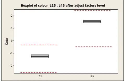
[image:6.595.305.545.200.356.2]The process settings for all influential variables are shown in Table 5. The performance after 1 cycle of the improvement can be explained by the box plots in Fig. 11. These results show that the performance of the new settings under the basic linear regression element of CRSO method seems superior to the previous levels. The new levels of decision variables also bring the 70 % reduction on the paint repairs cost and improve first time quality from 70% to 88%.
Fig. 11 Two Independent Box Plot Comparisons showing the Performance of the Mean Responses and the Standard
Deviation of L15 and L45 Responses.
As stated earlier, the experiments in this research was restricted to only one cycle. Consequently conclusions may not be optimal. Other stochastic approaches could be extended to the method based on conventional factorial designs to compare its performance, especially in terms of speed of convergence, and when the error standard deviation is at higher levels. Other stochastic approaches could be extended to the method based on conventional factorial designs to compare its performance, especially in terms of speed of convergence, and when the error standard deviation is at higher levels.
REFERENCES
[1] FANUC Robotics Manual Available: www.fanucrobotics.com [2] R.H. Myers and D.C. Montgomery, Response Surface Methodology:
Process and Product Optimisation using Designed Experiments, John
Wiley & Sons, Inc, 1995.
[3] G.E.P. Box and K.B. Wilson, “On the Experimental Attainment of Optimum Conditions,” Journal of the Royal Statistical Society, Series. B, vol. 13, 1951, pp. 1-45.
[4] G.E.P. Box and N.R. Draper, “Evolutionary Operation, A Statistical
Method for Process Improvement,” John Wiley & Sons, Inc, 1969.
[5] G.E.P. Box, “Evolutionary Operation: a Method for Increasing Industrial Productivity,” Applied Statistics, vol. 6, 1957, pp. 81-101.
[6] D.C. Montgomery, Design and Analysis of Experiments, John Wiley & Sons, Inc, 1991.
[7] P.Luangpaiboon, “Proposed Finishing Strategies Based on Experimental Designs for Process Optimisation,” Thammasat International Journal of
Science and Technology, pp. 39-45, 2001.
[8] P. Luangpaiboon and P. Sermpattarachai, “Response Surface Optimisation via Steepest Ascent, Simulated Annealing and Ant Colony Optimisation Algorithms,” Proceedings of the DSI International
Conference 2007, Bangkok, Thailand, 2007.
Da
ta
L45 L15
2
1
0
-1
-2