Structured Penalties for Log-linear Language Models
Anil Nelakanti,*‡C´edric Archambeau,*Julien Mairal,†Francis Bach,‡Guillaume Bouchard*
*Xerox Research Centre Europe, Grenoble, France
†INRIA-LEAR Project-Team, Grenoble, France ‡
INRIA-SIERRA Project-Team, Paris, France
[email protected] [email protected]
Abstract
Language models can be formalized as log-linear regression models where the input fea-tures represent previously observed contexts up to a certain length m. The complexity of existing algorithms to learn the parameters by maximum likelihood scale linearly innd, where nis the length of the training corpus anddis the number of observed features. We present a model that grows logarithmically ind, making it possible to efficiently leverage longer contexts. We account for the sequen-tial structure of natural language using tree-structured penalized objectives to avoid over-fitting and achieve better generalization.
1 Introduction
Language models are crucial parts of advanced nat-ural language processing pipelines, such as speech recognition (Burget et al., 2007), machine trans-lation (Chang and Collins, 2011), or information retrieval (Vargas et al., 2012). When a sequence of symbols is observed, a language model pre-dicts the probability of occurrence of the next sym-bol in the sequence. Models based on so-called back-off smoothing have shown good predictive power (Goodman, 2001). In particular, Kneser-Ney (KN) and its variants (Kneser and Ney, 1995) are still achieving state-of-the-art results for more than a decade after they were originally proposed. Smooth-ing methods are in fact clever heuristics that require tuning parameters in an ad-hoc fashion. Hence, more principled ways of learning language mod-els have been proposed based on maximum en-tropy (Chen and Rosenfeld, 2000) or conditional
random fields (Roark et al., 2004), or by adopting a Bayesian approach (Wood et al., 2009).
In this paper, we focus on penalized maxi-mum likelihood estimation in log-linear models. In contrast to language models based on unstruc-tured norms such as `2 (quadratic penalties) or
`1 (absolute discounting), we use tree-structured
norms (Zhao et al., 2009; Jenatton et al., 2011). Structured penalties have been successfully applied to various NLP tasks, including chunking and named entity recognition (Martins et al., 2011), but not lan-guage modelling. Such penalties are particularly well-suited to this problem as they mimic the nested nature of word contexts. However, existing optimiz-ing techniques are not scalable for large contextsm.
In this work, we show that structured tree norms provide an efficient framework for language mod-elling. For a special case of these tree norms, we obtain an memory-efficient learning algorithm for log-linear language models. Furthermore, we aslo give the first efficient learning algorithm for struc-tured `∞ tree norms with a complexity nearly
lin-ear in the number of training samples. This leads to a memory-efficientandtime-efficient learning algo-rithm for generalized linear language models.
The paper is organized as follows. The model and other preliminary material is introduced in Sec-tion 2. In SecSec-tion 3, we review unstructured penal-ties that were proposed earlier. Next, we propose structured penalties and compare their memory and time requirements. We summarize the characteris-tics of the proposed algorithms in Section 5 and ex-perimentally validate our findings in Section 6.
3
4
6
6
5 7
7
7
(a) Trie-structured vector.
w= [3 4 6 6 4 5 7 7]>.
3
4
6 [2]
4 5
7 [2]
(b) Tree-structured vector.
w= [3 4 6 6 4 5 7 7]>.
2.8
3.5
4.8
4.3
2.3 3
5.6
4.9
(c)`T
2-proximalΠ`T
2
(w,0.8) =
[2.8 3.5 4.8 4.3 2.3 3 5.6 4.9]>.
3
4
5.2 [2]
3.2 4.2
5.4 [2]
(d) `T
∞-proximalΠ`T
[image:2.612.81.538.62.261.2]∞(w,0.8) = [3 4 5.2 5.2 3.2 4.2 5.4 5.4]>.
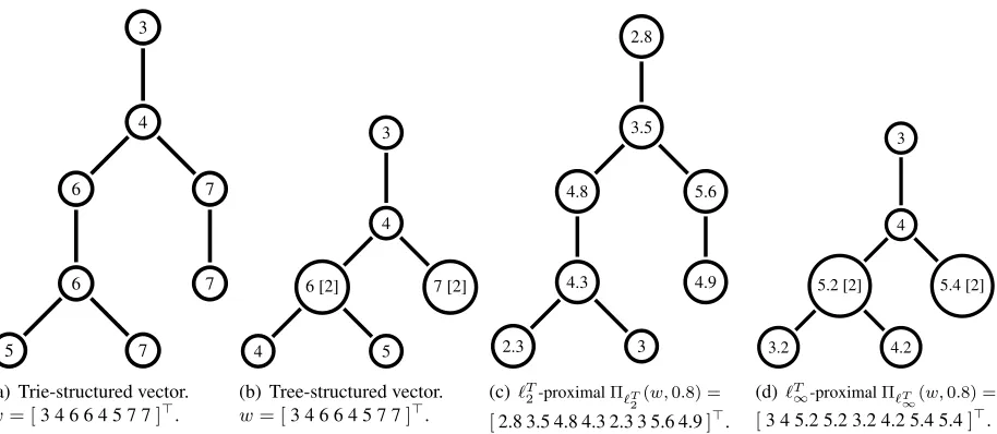
Figure 1: Example of uncollapsed (trie) and corresponding collapsed (tree) structured vectors and proximal operators applied to them. Weight values are written inside the node. Subfigure (a) shows the complete trieS and Subfigure (b) shows the corresponding collapsed treeT. The number in the brackets shows the number of nodes collapsed. Subfigure (c) shows vector after proximal projection for`T2-norm (which cannot be collapsed), and Subfigure (d) that of`T∞-norm proximal projection which can be collapsed.
2 Log-linear language models
Multinomial logistic regression and Poisson regres-sion are examples of log-linear models (McCullagh and Nelder, 1989), where the likelihood belongs to an exponential family and the predictor is lin-ear. The application of log-linear models to lan-guage modelling was proposed more than a decade ago (Della Pietra et al., 1997) and it was shown to be competitive with state-of-the-art language mod-elling such as Knesser-Ney smoothing (Chen and Rosenfeld, 2000).
2.1 Model definition
Let V be a set of words or more generally a set of symbols, which we call vocabulary. Further, letxy
be a sequence ofn+ 1symbols ofV, wherex∈Vn andy∈V. We model the probability that symboly
succeedsxas
P(y=v|x) = e
w>
vφm(x)
P
u∈V ew
>
uφm(x)
, (1)
whereW = {wv}v∈V is the set of parameters, and
φm(x)is the vector of features extracted fromx, the sequence precedingy. We will describe the features shortly.
Let x1:i denote the subsequence ofx starting at the first position up to theithposition andyithe next symbol in the sequence. Parameters are estimated by minimizing the penalized log-loss:
W∗ ∈argmin
W∈K
f(W) +λΩ(W), (2)
wheref(W) := −Pn
i=1lnp(yi|x1:i;W)and Kis a convex set representing the constraints applied on the parameters. Overfitting is avoided by adjust-ing the regularization parameter λ, e.g., by cross-validation.
2.2 Suffix tree encoding
Algorithm 1 W∗ := argmin {f(X, Y;W)+ λΩ(W)}Stochastic optimization algorithm (Hu et al., 2009)
1 Input: λregularization parameter ,LLipschitz constant of ∇f,µcoefficient of strong-convexity off+λΩ,Xdesign matrix,Y label set
2 Initialize:W=Z= 0,τ=δ= 1,ρ=L+µ
3 repeat until maximum iterations 4 #estimate point for gradient update
W = (1−τ)W+τ Z
5 #use mini-batch{Xϑ, Yϑ}for update
W= ParamUpdate(Xϑ, Yϑ, W , λ, ρ) 6 #weighted combination of estimates
Z= 1
ρτ+µ (1−µ)Z+ (µ−ρ)W+ρW
7 #update constants
ρ=L+µ/δ,τ = √
4δ+δ2−δ
2 ,δ= (1−τ)δ
Procedure:W:= ParamUpdate(Xϑ, Yϑ, W , λ, ρ) 1 W0 =W−1
ρ∇f(Xϑ, Yϑ, W) #gradient step
2 W = [W]+ #projection to non-negative orthant
3 W = ΠΩ(w, κ) #proximal step
always observed in the same context, the successive suffixes are collapsed into a single node. The un-collapsed version of the suffix treeT is called a suf-fixtrie, which we denoteS. A suffix trie also has a tree structure, but it potentially has much larger number of nodes. An example of a suffix trieSand the associated suffix treeT are shown in Figures 1(a) and 1(b) respectively. We use|S|to denote the num-ber of nodes in the trieSand|T|for the number of nodes in the treeT.
Suffix tree encoding is particularly helpful in ap-plications where the resulting hierarchical structures are thin and tall with numerous non-branching paths. In the case of text, it has been observed that the num-ber of nodes in the tree grows slower than that of the trie with the length of the sequence (Wood et al., 2011; Kennington et al., 2012). This is a signif-icant gain in the memory requirements and, as we will show in Section 4, can also lead to important computational gains when this structure is exploited. The feature vector φm(x) encodes suffixes (or contexts) of increasing length up to a maximum lengthm. Hence, the model defined in (1) is simi-lar tom-gram language models. Naively, the feature vectorφm(x) corresponds to one path of lengthm starting at the root of the suffix trieS. The entries inW correspond to weights for each suffix. We thus have a trie structureSonW (see Figure 1(a))
con-straining the number of free parameters. In other words, there is one weight parameter per node in the trieSand the matrix of parametersW is of size|S|. In this work, however, we consider models where the number of parameters is equal to the size of the suffix treeT, which has much fewer nodes thanS. This is achieved by ensuring that all parameters cor-responding to suffixes at a node share the same pa-rameter value (see Figure 1(b)). These papa-rameters correspond to paths in the suffix trie that do not branchi.e.sequence of words that always appear to-gether in the same order.
2.3 Proximal gradient algorithm
The objective function (2) involves a smooth convex lossf and a possibly non-smooth penaltyΩ. Sub-gradient descent methods for non-smooth Ωcould be used, but they are unfortunately very slow to con-verge. Instead, we choose proximal methods (Nes-terov, 2007), which have fast convergence rates and can deal with a large number of penalties Ω, see (Bach et al., 2012).
Proximal methods iteratively update the current estimate by making a generalized gradient update at each iteration. Formally, they are based on a lin-earization of the smooth functionfaround a param-eter estimate W, adding a quadratic penalty term to keep the updated estimate in the neighborhood ofW. At iterationt, the update of the parameterW
is given by
Wt+1= argmin
W∈K n
f(W) + (W −W)>∇f(W)
+Ω(W) + L
2kW −Wk
2 2
, (3)
where L > 0 is an upper-bound on the Lipschitz constant of the gradient∇f. The matrixW could either be the current estimate Wt or its weighted combination with the previous estimate for accel-erated convergence depending on the specific algo-rithm used (Beck and Teboulle, 2009). Equation (3) can be rewritten to be solved in two independent steps: a gradient update from the smooth part fol-lowed by a projection depending only on the non-smooth penalty:
W0 =W − 1
Wt+1= argmin
W∈K 1 2
W −W0
2 2+
λΩ(W) L . (5)
Update (5) is called the proximal operator of W0
with parameter Lλ that we denote ΠΩ W0,λL
. Ef-ficiently computing the proximal step is crucial to maintain the fast convergence rate of these methods.
2.4 Stochastic proximal gradient algorithm
In language modelling applications, the number of training samplesn is typically in the range of105
or larger. Stochastic version of the proximal meth-ods (Hu et al., 2009) have been known to be well adapted when n is large. At every update, the stochastic algorithm estimates the gradient on a mini-batch, that is, a subset of the samples. The size of the mini-batches controls the trade-off between the variance in the estimate of gradient and the time required for compute it. In our experiments we use mini-batches of size 400. The training algorithm is summarized in Algorithm 1. The acceleration is ob-tained by making the gradient update at a specific weighted combination of the current and the previ-ous estimates of the parameters. The weighting is shown in step 6 of the Algorithm 1.
2.5 Positivity constraints
Without constraining the parameters, the memory required by a model scales linearly with the vocabu-lary size|V|. Any symbol inV observed in a given context is a positive example, while any symbols inV that does not appear in this context is a neg-ative example. When adopting a log-linear language model, the negative examples are associated with a small negative gradient step in (4), so that the solu-tion is not sparse accross multiple categories in gen-eral. By constraining the parameters to be positive (i.e., the set of feasible solutions K is the positive orthant), the projection step 2 in Algorithm 1 can be done with the same complexity, while maintaining sparse parameters accross multiple categories. More precisely, the weights for the categoryk associated to a given contextx, is always zeros if the categoryk
never occured after contextx. A significant gain in memory (nearly|V|-fold for large context lengths) was obtained without loss of accuracy in our exper-iments.
3 Unstructured penalties
Standard choices for the penalty functionΩ(W) in-clude the `1-norm and the squared `2-norm. The
former typically leads to a solution that is sparse and easily interpretable, while the latter leads to a non-sparse, generally more stable one. In partic-ular, the squared`2 and `1 penalties were used in
the context of log-linear language models (Chen and Rosenfeld, 2000; Goodman, 2004), reporting perfor-mances competitive with bi-gram and tri-gram inter-polated Kneser-Ney smoothing.
3.1 Proximal step on the suffix trie
For squared `2 penalties, the proximal step
Π`2 2(w
t,κ
2)is the element-wise rescaling operation:
w(it+1)←w(it)(1 +κ)−1 (6)
For`1penalties, the proximal stepΠ`1(w
t, κ)]is the
soft-thresholding operator:
wi(t+1)←max(0, w(it)−κ). (7)
These projections have linear complexity in the number of features.
3.2 Proximal step on the suffix tree
When feature values are identical, the corresponding proximal (and gradient) steps are identical. This can be seen from the proximal steps (7) and (6), which apply to single weight entries. This property can be used to group together parameters for which the fea-ture values are equal. Hence, we can collapse suc-cessive nodes that always have the same values in a suffix trie (as in Figure 1(b)), that is to say we can directly work on the suffix tree. This leads to a prox-imal step with complexity that scales linearly with the number of symbols seen in the corpus (Ukkonen, 1995) and logarithmically with context length.
4 Structured penalties
The`1 and squared`2 penalties do not account for
Algorithm 2w := Π`T
2(w, κ) Proximal projection
step for`T2 on groupingG.
1 Input: T suffix tree,wtrie-structured vector,κthreshold 2 Initialize:{γi}= 0,{ηi}= 1
3 η= UpwardPass(η, γ, κ, w) 4 w= DownwardPass(η, w)
Procedure:η:= UpwardPass(η, γ, κ, w) 1 forx∈DepthFirstSuffixTraversal(T,PostOrder) 2 γx=w2x+
P
h∈children(x)γh
3 ηx= [1−κ/√γx]+
4 γx=η2 xγx
Procedure:w:= DownwardPass(η, w) 1 forx∈DepthFirstSuffixTraversal(T,PreOrder) 2 wx=ηxwx
3 forh∈children(x)
4 ηh=ηxηh
a DepthFirstSuffixTraversal(T,Order) returns observed suf-fixes from the suffix treeTby depth-first traversal in the order prescribed byOrder.
b wx is the weights corresponding to the suffixx from the weight vectorwandchildren(x)returns all the immediate children to suffixxin the tree.
norms (Zhao et al., 2009; Jenatton et al., 2011), which are based on the suffix trie or tree, where sub-trees correspond to contexts of increasing lengths. As will be shown in the experiments, this prevents the model to overfit unlike the `1- or squared `2
-norm.
4.1 Definition of tree-structured`Tp norms
Definition 1. Letx be a training sequence. Group
g(w, j) is the subvector of w associated with the subtree rooted at the nodejof the suffix trieS(x).
Definition 2. LetGdenote the ordered set of nodes of the tree T(x) such that for r < s, g(w, r)∩ g(w, s) = ∅ or g(w, r) ⊂ g(w, s). The tree-structured`p-norm is defined as follows:
`Tp(w) =X
j∈G
kg(w, j)kp. (8)
We specifically consider the casesp = 2,∞ for which efficient optimization algorithms are avail-able. The `Tp-norms can be viewed as a group sparsity-inducing norms, where the groups are or-ganized in a tree. This means that when the weight associated with a parent in the tree is driven to zero, the weights associated to all its descendants should also be driven to zero.
Algorithm 3w := Π`T
∞(w, κ)Proximal projection step for`T
∞on groupingG.
Input: T suffix tree,w=[v c]tree-structured vectorv with corresponding number of suffixes collapsed at each node in
c,κthreshold
1 forx∈DepthFirstNodeTraversal(T,PostOrder) 2 g(v, x) :=π`T
∞(g(v, x), cxκ)
Procedure:q:=π`∞(q, κ)
Input:q= [v c], qi= [vici], i= 1,· · ·,|q| Initialize:U={}, L={}, I={1,· · ·,|q|} 1 whileI6=∅
2 pick randomρ∈I #choose pivot 3 U={j|vj≥vρ} #larger thanvρ
4 L={j|vj< vρ} #smaller thanvρ
5 δS=P
i∈Uvi·ci, δC= P
i∈Uci
6 if(S+δS)−(C+δC)ρ < κ
7 S:= (S+δS), C:= (C+δC), I:=L
8 elseI:=U\{ρ} 9 r=S−κ
C ,vi:=vi−max(0, vi−r) #take residuals
a DepthFirstNodeTraversal(T,Order) returns nodesxfrom the suffix treeT by depth-first traversal in the order prescribed byOrder.
For structured `Tp-norm, the proximal step amounts to residuals of recursive projections on the
`q-ball in the order defined by G (Jenatton et al., 2011), where`q-norm is the dual norm of`p-norm1. In the case`T2-norm this comes to a series of pro-jections on the `2-ball. For `T∞-norm it is instead
projections on the`1-ball. The order of projections
defined byG is generated by an upward pass of the suffix trie. At each node through the upward pass, the subtree below is projected on the dual norm ball of sizeκ, the parameter of proximal step. We detail the projections on the norm ball below.
4.2 Projections on`q-ball forq= 1,2
Each of the above projections on the dual norm ball takes one of the following forms depending on the choice of the norm. Projection of vectorw on the
`2-ball is equivalent to thresholding the magnitude
ofwbyκunits while retaining its direction:
w←[||w||2−κ]+
w ||w||2
. (9)
This can be performed in time linear in size ofw,
O(|w|). Projection of a non-negative vectorwon the
`1-ball is more involved and requires thresholding
1`p
by a value such that the entries in the resulting vector add up toκ, otherwisewremains the same:
w←[w−τ]+s.t.||w||1=κorτ = 0. (10)
τ = 0 is the case where w lies inside the `1-ball
of sizeκwith||w||1 < κ, leavingwintact. In the
other case, the threshold τ is to be computed such that after thresholding, the resulting vector has an
`1-norm of κ. The simplest way to achieve this is
to sort by descending order the entriesw=sort(w)
and pick theklargest values such that the(k+ 1)th
largest entry is smaller thanτ:
k
X
i=1
wi−τ =κandτ > wk+1. (11)
We refer towkas the pivot and are only interested in entries larger than the pivot. Given a sorted vector, it requires looking up to exactlykentries, however, sorting itself takeO(|w|log|w|).
4.3 Proximal step
Naively employing the projection on the`2-ball
de-scribed above leads to an O(d2) algorithm for `T2
proximal step. This could be improved to a linear al-gorithm by aggregating all necessary scaling factors while making an upward pass of the trieS and ap-plying them in a single downward pass as described in (Jenatton et al., 2011). In Algorithm 2, we detail this procedure for trie-structured vectors.
The complexity of `T∞-norm proximal step de-pends directly on that of the pivot finding algorithm used within its`1-projection method. Naively
sort-ing vectors to find the pivot leads to anO(d2logd)
algorithm. Pivot finding can be improved by ran-domly choosing candidates for the pivot and the best known algorithm due to (Bruckner, 1984) has amortized linear time complexity in the size of the vector. This leaves us with O(d2) complexity for
`T∞-norm proximal step. (Duchi et al., 2008) pro-poses a method that scales linearly with the num-ber of non-zero entries in the gradient update (s)
but logarithmically in d. But recursive calls to
`1-projection over subtrees will fail the sparsity
assumption (withs ≈ d) making proximal step quadratic. Procedure forΠ`T
∞on trie-structured vec-tors using randomized pivoting method is described in Algorithm 3.
We next explain how the number of`1-projections
can be reduced by switching to the treeT instead of trieSwhich is possible due to the good properties of
`T∞-norm. Then we present a pivot finding method that is logarithmic in the feature size for our appli-cation.
4.4 `T
∞-norm with suffix trees
We consider the case where all parameters are ini-tialized with the same value for the optimization pro-cedure, typically with zeros. The condition that the parameters at any given node continue to share the same value requires that both the gradient update (4) and proximal step (5) have this property. We mod-ify the tree structure to ensure that after gradient up-dates parameters at a given node continue to share a single value. Nodes that do not share a value after gradient update are split into multiple nodes where each node has a single value. We formally define this property as follows:
Definition 3. Aconstant value non-branching path
is a set of nodesP ∈ P(T, w)of a tree structureT
w.r.t. vectorwifP has|P|nodes with|P| −1edges between them and each node has at most one child and all nodesi, j ∈P have the same value in vector
waswi =wj.
The nodes of Figure 1(b) correspond to constant value non-branching paths when the values for all parameters at each of the nodes are the same. Next we show that this tree structure is retained after proximal steps of`T∞-norm.
Proposition 1. Constant value non-branching paths
P(T, w)ofT structured vectorware preserved un-der the proximal projection stepΠ`T
∞(w, κ). Figure 1(d) illustrates this idea showing`T∞ pro-jection applied on the collapsed tree. This makes it memory efficient but the time required for the prox-imal step remains the same since we must project each subtree of S on the `1-ball. The sequence of
projections at nodes of S in a non-branching path can be rewritten into a single projection step using the following technique bringing the number of pro-jections from|S|to|T|.
Proposition 2. Successive projection steps for sub-trees with root in a constant value non-branching pathP ={g1,· · ·, g|P|} ∈ P(T, w)forΠ`T
isπg|P|◦ · · · ◦πg1(w, κ)applied in bottom-up order
defined byG. The composition of projections can be rewritten into a single projection step withκscaled by the number of projections|P|as,
πg|P|(w, κ|P|)≡πg|P|◦ · · · ◦πg1(w, κ).
The above propositions show that`T∞-norm can be used with the suffix tree with fewer projection steps. We now propose a method to further improve each of these projection steps.
4.5 Fast proximal step for`T
∞-norm
Let k be the cardinality of the set of values larger than the pivot in a vector to compute the thresh-old for`1-projection as referred in (11). This value
varies from one application to another, but for lan-guage applications, our experiments on 100K en-glish words (APNews dataset) showed thatkis gen-erally small: its value is on average 2.5, and its maximum is around 10 and 20, depending on the regularization level. We propose using a max-heap data structure (Cormen et al., 1990) to fetch thek -largest values necessary to compute the threshold. Given the heap of the entries the cost of finding the pivot isO(klog(d))if the pivot is thekthlargest en-try and there are dfeatures. This operation is per-formeddtimes for`T∞-norm as we traverse the tree bottom-up. The heap itself is built on the fly dur-ing this upward pass. At each subtree, the heap is built by merging those of their children in constant time by using Fibonacci heaps. This leaves us with a
O(dklog(d))complexity for the proximal step. This procedure is detailed in Algorithm 4.
[image:7.612.310.531.97.345.2]5 Summary of the algorithms
Table 1 summarizes the characteristics of the algo-rithms associated to the different penalties:
1. The unstructured norms `p do not take into account the varying sparsity level with con-text length. For p=1, this leads to a sparse solution and for p=2, we obtain the classical quadratic penalty. The suffix tree representa-tion leads to an efficient memory usage. Fur-thermore, to make the training algorithm time efficient, the parameters corresponding to con-texts which always occur in the same larger
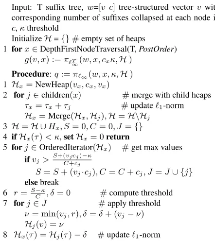
Algorithm 4w := Π`T
∞(w, κ)Proximal projection step for`T
∞on groupingGusing heap data structure. Input: T suffix tree,w=[v c]tree-structured vectorv with corresponding number of suffixes collapsed at each node in
c,κthreshold
InitializeH={}#empty set of heaps 1 forx∈DepthFirstNodeTraversal(T,PostOrder)
g(v, x) :=π`T
∞(w, x, cxκ,H)
Procedure:q:=π`∞(w, x, κ,H) 1 Hx=NewHeap(vx, cx, vx)
2 forj∈children(x) #merge with child heaps
τx=τx+τj #update`1-norm
Hx=Merge(Hx,Hj),H=H\Hj
3 H=H ∪Hx, S= 0, C= 0, J={} 4 ifHx(τ)< κ,setHx= 0return
5 forj∈OrderedIterator(Hx) #get max values
ifvj>S+(vj·cj)−κ
C+cj
S=S+ (vj·cj), C=C+cj, J=J∪ {j}
elsebreak 6 r= S−κ
C , δ= 0 #compute threshold
7 forj∈J #apply threshold
ν= min(vj, r), δ=δ+ (vj−ν) Hj(v) =ν
8 Hx(τ) =Hj(τ)−δ #update`1-norm
a. Heap structure on vectorwholds three values(v, c, τ)at each node.v, cbeing value and its count,τis the`1-norm of
the sub-vector below. Tuples are ordered by decreasing value ofvandHjrefers to heap with values in sub-tree rooted at j. Merge operation merges the heaps passed. OrderedIterator returns values from the heap in decreasing order ofv.
context are grouped. We will illustrate in the experiments that these penalties do not lead to good predictive performances.
2. The`T2-norm nicely groups features by subtrees which concurs with the sequential structure of sequences. This leads to a powerful algorithm in terms of generalization. But it can only be applied on the uncollapsed tree since there is no closure property of theconstant value non-branching pathfor its proximal step making it less amenable for larger tree depths.
3. The`T∞-norm groups features like the`T2-norm while additionally encouraging numerous fea-ture groups to share a single value, leading to a substantial reduction in memory usage. The generalization properties of this algorithm is as good as the generalization obtained with the`T2
Penalty good generalization memory efficient time efficient unstructured`1and`22 no yesO(|T|) yesO(|T|)
struct.
`T2 yes noO(|S|) noO(|S|)
`T∞ rand. pivot yes yesO(|T|) noO(|T|2)
[image:8.612.126.487.65.135.2]`T∞ heap yes yesO(|T|) yesO(|T|log|T|)
Table 1: Properties of the algorithms proposed in this paper. Generalization properties are as compared by their performance with increasing context length. Memory efficiency is measured by the number of free parameters ofW in the optimization. Note that the suffix tree is much smaller than the trie (uncollapsed tree):|T|<<|S|. Time complexities reported are that of one proximal projection step.
2 4 6 8 10 12
210 220 230 240 250 260
order of language model
p
e
r
p
le
x
it
y
KN
`2
2
`1
`T
2
`T
∞
(a) Unweighted penalties.
2 4 6 8 10 12
210 220 230 240 250 260
order of language model
p
e
r
p
le
x
it
y
K N w`2 2
w`
1
w`T 2
w`T ∞
(b) Weighted penalties.
2 4 6 8 10 12
0 2 4 6 8x 10
5
order of language model
#
o
f
p
a
r
a
m
e
t
e
r
s
K N w`T
2
w`T ∞
(c) Model complexity for structured penalties.
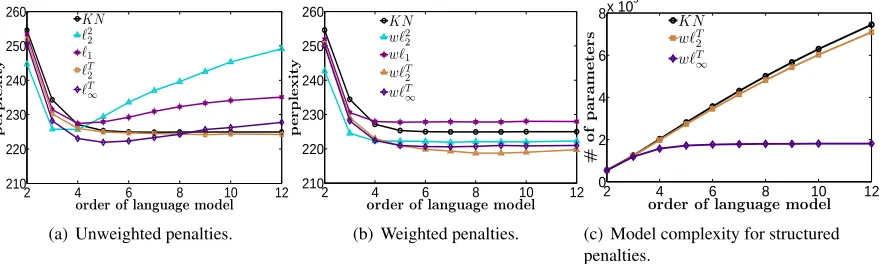
Figure 2: (a) compares average perplexity (lower is better) of different methods from2-gram through 12 -gram on four different 100K-20K train-test splits. (b) plot compares the same with appropriate feature weighting. (c) compares model complexity for weighted structured penaltiesw`T2 and w`T∞ measure by then number of parameters.
means that the proximal step can be applied di-rectly to the suffix tree. There is thus also a significant gain of performances.
6 Experiments
In this section, we demonstrate empirically the prop-erties of the algorithms summarized in Table 1. We consider four distinct subsets of the Associated Press News (AP-news) text corpus with train-test sizes of 100K-20K for our experiments. The corpus was preprocessed as described in (Bengio et al., 2003) by replacing proper nouns, numbers and rare words with special symbols “hproper nouni”, “#n” and “hunknowni” respectively. Punctuation marks are retained which are treated like other normal words. Vocabulary size for each of the training subsets was around 8,500 words. The model was reset at the start of each sentence, meaning that a word in any given sentence does not depend on any word in the previ-ous sentence. The regularization parameterλis
cho-sen for each model by cross-validation on a smaller subset of data. Models are fitted to training sequence of 30K words for different values ofλand validated against a sequence of 10K words to chooseλ.
We quantitatively evaluate the proposed model using perplexity, which is computed as follows:
P({xi, yi}, W) = 10 n
−1 nV
Pn
i=1I(yi∈V) logp(yi|x1:i;W) o
,
wherenV = PiI(yi ∈ V). Performance is mea-sured for varying depth of the suffix trie with dif-ferent penalties. Interpolated Kneser-Ney results were computed using the openly available SRILM toolkit (Stolcke, 2002).
Figure 2(a) shows perplexity values averaged over four data subsets as a function of the language model order. It can be observed that performance of un-structured`1and squared`2penalties improve until
a relatively low order and then degrade, while `T2
[image:8.612.88.528.216.348.2]2 4 6 8 10 12 20
40 60
tree depth
ti
m
e
(s
e
c
)
rand-pivot rand-pivot-col
(a) Iteration time of random-pivoting on the collapsed and uncollapsed trees.
1 2 3 4 5
x 106 20
40 60
train size
ti
m
e
(s
e
c
)
k-best heap rand-pivot-col
(b) Iteration time of random-pivoting and
[image:9.612.150.466.61.204.2]k-best heap on the collapsed tree.
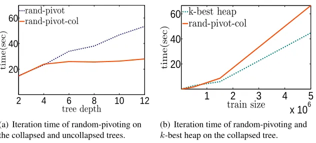
Figure 3: Comparison of different methods for performing `T∞ proximal projection. The rand-pivot is the random pivoting method of (Bruckner, 1984) andrand-pivot-colis the same applied with the nodes collapsed. Thek-best heapis the method described in Algorithm 4.
that taking the tree-structure into account is benefi-cial. Moreover, the log-linear language model with
`T2 penalty performs similar to interpolated Kneser-Ney. The `T∞-norm outperforms all other models at order 5, but taking the structure into account does not prevent a degradation of the performance at higher orders, unlike`T
2. This means that a single
regularization for all model orders is still inappro-priate.
To investigate this further, we adjust the penal-ties by choosing an exponential decrease of weights varying asαm for a feature at depthmin the suffix tree. Parameterαwas tuned on a smaller validation set. The best performing values for these weighted models w`22, w`1, w`2T and w`T∞ are 0.5, 0.7, 1.1
and 0.85 respectively. The weighting scheme fur-ther appropriates the regularization at various levels to suit the problem’s structure. Perplexity plots for weighted models are shown in Figure 2(b). While
w`1 improves at larger depths, it fails to compare
to others showing that the problem does not admit sparse solutions. Weighted `22 improves consider-ably and performs comparconsider-ably to the unweighted tree-structured norms. However, the introduction of weighted features prevents us from using the suf-fix tree representation, making these models inef-ficient in terms of memory. Weighted `T∞ is cor-rected for overfitting at larger depths andw`T2 gains more than others. Optimal values for α are frac-tional for all norms exceptw`T2-norm showing that the unweighted model`T2-norm was over-penalizing features at larger depths, while that of others were
under-penalizing them. Interestingly, perplexity im-proves up to about 9-grams with w`T2 penalty for the data set we considered, indicating that there is more to gain from longer dependencies in natural language sentences than what is currently believed.
Figure 2(c) compares model complexity mea-sured by the number of parameters for weighted models using structured penalties. The `T2 penalty is applied on trie-structured vectors, which grows roughly at a linear rate with increasing model order. This is similar to Kneser-Ney. However, the number of parameters for thew`T∞ penalty grows logarith-mically with the model order. This is due to the fact that it operates on the suffix tree-structured vectors instead of the suffix trie-structured vectors. These results are valid for, both, weighted and unweighted penalties.
increasing size of training data.
7 Conclusion
In this paper, we proposed several log-linear lan-guage models. We showed that with an efficient data structure and structurally appropriate convex regularization schemes, they were able to outper-form standard Kneser-Ney smoothing. We also de-veloped a proximal projection algorithm for the tree-structured`T∞-norm suitable for large trees.
Further, we showed that these models can be trained online, that they accurately learn the m-gram weights and that they are able to better take advan-tage of long contexts. The time required to run the optimization is still a concern. It takes 7583 min-utes on a standard desktop computer for one pass of the of the complete AP-news dataset with 13 mil-lion words which is little more than time reported for (Mnih and Hinton, 2007). The most time con-suming part is computing the normalization factor for the log-loss. A hierarchical model in the flavour of (Mnih and Hinton, 2008) should lead to signifi-cant improvements to this end. Currently, the com-putational bottleneck is due to the normalization fac-tor in (1) as it appears in every gradient step com-putation. Significant savings would be obtained by computing it as described in (Wu and Khundanpur, 2000).
Acknowledgements
The authors would like to thank anonymous review-ers for their comments. This work was partially supported by the CIFRE grant 1178/2010 from the French ANRT.
References
F. Bach, R. Jenatton, J. Mairal, and G. Obozinski. 2012. Optimization with sparsity-inducing penalties.
Foun-dations and Trends in Machine Learning, pages 1–
106.
A. Beck and M. Teboulle. 2009. A fast itera-tive shrinkage-thresholding algorithm for linear in-verse problems. SIAM Journal of Imaging Sciences, 2(1):183–202.
Y. Bengio, R. Ducharme, P. Vincent, and C. Jauvin. 2003. A neural probabilistic language model.Journal of
Ma-chine Learning Research, 3:1137–1155.
P. Bruckner. 1984. An o(n) algorithm for quadratic knapsack problems. Operations Research Letters, 3:163–166.
L. Burget, P. Matejka, P. Schwarz, O. Glembek, and J.H. Cernocky. 2007. Analysis of feature extraction and channel compensation in a GMM speaker recognition system. IEEE Transactions on Audio, Speech and
Language Processing, 15(7):1979–1986, September.
Y-W. Chang and M. Collins. 2011. Exact decoding of phrase-based translation models through lagrangian relaxation. InProc. Conf. Empirical Methods for Nat-ural Language Processing, pages 26–37.
S. F. Chen and R. Rosenfeld. 2000. A survey of smoothing techniques for maximum entropy models.
IEEE Transactions on Speech and Audio Processing,
8(1):37–50.
T. H. Cormen, C. E. Leiserson, and R. L. Rivest. 1990.
An Introduction to Algorithms. MIT Press.
S. Della Pietra, V. Della Pietra, and J. Lafferty. 1997. Inducing features of random fields. IEEE Transac-tions on Pattern Analysis and Machine Intelligence, 19(4):380–393.
J. Duchi, S. Shalev-Shwartz, Y. Singer, and T. Chandra. 2008. Efficient projections onto the`1-ball for
learn-ing in high dimensions.Proc. 25th Int. Conf. Machine Learning.
R. Giegerich and S. Kurtz. 1997. From ukkonen to Mc-Creight and weiner: A unifying view of linear-time suffix tree construction.Algorithmica.
J. Goodman. 2001. A bit of progress in language mod-elling. Computer Speech and Language, pages 403– 434, October.
J. Goodman. 2004. Exponential priors for maximum en-tropy models. InProc. North American Chapter of the Association of Computational Linguistics.
C. Hu, J.T. Kwok, and W. Pan. 2009. Accelerated gra-dient methods for stochastic optimization and online learning. Advances in Neural Information Processing Systems.
R. Jenatton, J. Mairal, G. Obozinski, and F. Bach. 2011. Proximal methods for hierarchical sparse cod-ing. Journal of Machine Learning Research, 12:2297– 2334.
C. R. Kennington, M. Kay, and A. Friedrich. 2012. Sufx trees as language models. Language Resources and Evaluation Conference.
R. Kneser and H. Ney. 1995. Improved backing-off for m-gram language modeling. InProc. IEEE Int. Conf. Acoustics, Speech and Signal Processing, volume 1. A. F. T. Martins, N. A. Smith, P. M. Q. Aguiar, and
M. A. T. Figueiredo. 2011. Structured sparsity in structured prediction. InProc. Conf. Empirical
Meth-ods for Natural Language Processing, pages 1500–
P. McCullagh and J. Nelder. 1989. Generalized linear models. Chapman and Hall. 2nd edition.
A. Mnih and G. Hinton. 2007. Three new graphical mod-els for statistical language modelling. Proc. 24th Int.
Conference on Machine Learning.
A. Mnih and G. Hinton. 2008. A scalable hierarchical distributed language model. Advances in Neural In-formation Processing Systems.
Y. Nesterov. 2007. Gradient methods for minimizing composite objective function. CORE Discussion Pa-per.
B. Roark, M. Saraclar, M. Collins, and M. Johnson. 2004. Discriminative language modeling with con-ditional random fields and the perceptron algorithm.
Proc. Association for Computation Linguistics. A. Stolcke. 2002. Srilm- an extensible language
mod-eling toolkit. Proc. Int. Conf. Spoken Language Pro-cessing, 2:901–904.
E. Ukkonen. 1995. Online construction of suffix trees.
Algorithmica.
S. Vargas, P. Castells, and D. Vallet. 2012. Explicit rel-evance models in intent-oriented information retrieval diversification. InProc. 35th Int. ACM SIGIR Conf.
Research and development in information retrieval,
SIGIR ’12, pages 75–84. ACM.
F. Wood, C. Archambeau, J. Gasthaus, J. Lancelot, and Y.-W. Teh. 2009. A stochastic memoizer for sequence data. InProc. 26th Intl. Conf. on Machine Learning. F. Wood, J. Gasthaus, C. Archambeau, L. James, and
Y. W. Teh. 2011. The sequence memoizer. In
Com-munications of the ACM, volume 54, pages 91–98.
J. Wu and S. Khundanpur. 2000. Efficient training meth-ods for maximum entropy language modeling. Proc. 6th Inter. Conf. Spoken Language Technologies, pages 114–117.