Learning Constraints for Consistent Timeline Extraction
David McClosky and Christopher D. Manning Natural Language Processing Group
Computer Science Department Stanford University, Stanford, CA, USA {mcclosky,manning}@stanford.edu
Abstract
We present a distantly supervised system for extracting the temporal bounds of fluents (re-lations which only hold during certain times, such as attends school). Unlike previous pipelined approaches, our model does not as-sume independence between each fluent or even between named entities with known con-nections (parent, spouse, employer, etc.). In-stead, we model what makes timelines of flu-ents consistent by learning cross-fluent con-straints, potentially spanning entities as well. For example, our model learns that someone is unlikely to start a job at age two or to marry someone who hasn’t been born yet. Our sys-tem achieves a 36% error reduction over a pipelined baseline.
1 Introduction
Many information extraction (IE) systems tradition-ally extracted just relations, but a great many real world relations such as attends school or has spouse vary over time. To capture this, some recent IE systems have extended their focus from relations to
fluents (relations combined with temporal bounds).
This can be seen in the temporal slot filling track in the TAC-KBP 2011 shared task (Ji et al., 2011). A direct application of this work is the automatic im-provement of online resources such as Freebase and Wikipedia infoboxes. Indirect applications include question answering systems.
Fluents can be grouped together to form time-lines (see Figure 1 for an example) and provide eas-ily capturable consistency constraints. Our goal is
Figure 1: A timeline of two named entities. Each time span represents a fluent (a relation with temporal bounds). Temporal bounds are denoted by spans on the timeline. Fluents can create links between entities (e.g., marriage).
to learn these constraints and use them to produce more accurate timelines of significant events for people and organizations. For example, it is com-mon knowledge that someone cannot attend a school if they haven’t been born yet. Constraints on con-sistent timelines do not need to be hard constraints, though: it is rare, although possible, to become the CEO of a company at the age of 21.
Despite the rich constraints on valid timelines, there is relatively little work on exploiting these con-straints for mutual disambiguation. Many existing systems extract different parts of a timeline sepa-rately and use heuristics to combine them. These heuristics tend to optimize only local consistency (within a single fluent) but ignore more global con-straints across fluents (e.g., attending a school be-fore being born) or across fluents of two linked entities (e.g., attending a school before the school was founded). In this work, we explore using joint inference to enforce these constraints. We show that these techniques can yield substantial improve-ments. Additionally, our general approach is not specific to extracting temporal boundaries of fluents. It could easily be applied to other IE systems which
employ independent extractions followed by heuris-tics to improve consistency.
2 The timelining task
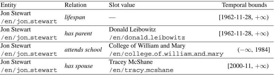
As a basis for our task, we first describe the Tempo-ral KBP task (Ji et al., 2011). As input, one is given a list of queries, a database of example fluents, and source documents. Queries are named entities (peo-ple or organizations) with their gold relations but no temporal bounds. The database consists of training entities with their fluents, including known tempo-ral bounds for each fluent. Example fluents can be seen in Table 1. Note that the database may be in-complete. In addition to missing fluents for an en-tity, some temporal bounds may be missing from the database; missing bounds are unfortunately in-distinguishable from unbounded ranges. As a result, we can only trust concrete temporal boundaries in the database. Source documents consist of raw text from news, blogs, and Wikipedia articles. For each fluent, systems must output their predicted temporal bounds, along with references to source documents to provide provenance.
Our task is a variation of the Temporal KBP task. In our case, the database is a collection of Freebase1 entities and their fluents, merged with Wikipedia in-foboxes. Each entity has a unique ID, allowing us to avoid some coreference issues (though there can still be issues in document retrieval). In Temporal KBP, the temporal representation allows for upper and lower bounds on both the event start and end: hsl, su, el, euiwheresl ≤start≤ su,el ≤end≤
eu. However, it is difficult to obtain these bounds
without manual annotation. As a result, we opted for the simpler representation which can be easily found in databases like Freebase. Our temporal represen-tation is limited to bounds of the formhstart, endi where either can be unbounded or unknown (both represented as±∞).
Our set of fluents is closely related to those in the Temporal KBP task. Our goal was to use as much temporal information as possible, with the hope of each fluent providing additional poten-tial constraints. While we omit the resides in and
member of fluents,2 we add several others. For
1
http://freebase.org
2
This is because these fluents are rarely present in Freebase
people and organizations, we add a special fluent,
lifespan, which doesn’t take a slot value.3 A list of fluents we use are listed in Table 3.
3 Model
To operate on a set of queries, we first collect can-didate temporal expression mentions for each fluent from our source documents. This limits us to us-ing temporal expression mentions which appear near fluent mentions in text. It also ensures that we can provide provenance for each temporal boundary as-sertion. This process is described in§3.1.
Our model contains two components, both of which assign probabilities to timelines. The
clas-sifier component determines how each candidate
temporal expression mention connects to its fluent (§3.2). For example, the mention may indicate the START of the fluent, theEND, both its START AND
END(for instantaneous events), or beUNRELATED. These connections involve relations between tempo-ral expression mentions and relations and we refer to them as metarelations.4 For features, the classifier uses the surrounding textual and syntactic context of temporal expression and fluent mentions. Each clas-sification decision is made independently, allowing for inconsistency at multiple levels (within a fluent, across fluents, or across entities). However, using joint inference, the classifier component can deter-mine the best overall span for each fluent.
The consistency component learns what makes timelines consistent (§3.3). It is similar in nature to a language model for timelines instead of sentences. Given a candidate timeline, the consistency compo-nent estimates its probability of occurring. This is done by decomposing timelines into a series of
ques-tions (such as “did the entity go to school before
starting a job?”) and learning the probabilities of different answers from training data.
Unlike the classifier component, the consistency component is blind to the underlying text in the source documents. The two components work to-gether to find a global timeline that is both based on textual evidence and coherent across entities using
with temporal bounds.
3
Note that this is a relation in the non-temporal KBP task.
4
Entity Relation Slot value Temporal bounds Jon Stewart
lifespan — [1962-11-28,+∞)
/en/jon stewart
Jon Stewart
has parent Donald Leibowitz [1962-11-28,+∞)
/en/jon stewart /en/donald leibowitz
Jon Stewart
attends school College of William and Mary (−∞, 1984]
/en/jon stewart /en/college of william and mary
Jon Stewart
has spouse Tracey McShane [2000-11,+∞)
[image:3.612.77.539.56.183.2]/en/jon stewart /en/tracy mcshane
Table 1: Example relations with their temporal bounds. Freebase IDs are shown inmonospace. Note that temporal bounds differ in their resolution (some are days of the year, others are only years). Some bounds are unknown (e.g., the start of the attends school fluent) and indistinguishable from unbounded. The lifespan fluent is a unary relation.
joint inference (note that they are trained indepen-dently). The inference process is described in§3.4.
3.1 Temporal expression retrieval
Given a fluent, we search for all textual mentions of the fluent and collect nearby temporal expression mentions. These temporal expressions are used as candidate boundaries for the fluent in later steps. The search process assumes that if a fluent’s entity and slot value co-occur in a sentence,5that sentence is typically a positive example of the fluent.6 This is sometimes known as distant supervision (Craven and Kumlien, 1999; Mintz et al., 2009). We use the Stanford Core NLP suite (Toutanova et al., 2003; Finkel et al., 2005; Klein and Manning, 2003; Lee et al., 2011) to annotate each document with POS and NER tags, parse trees, and coreference chains. On top of this, we apply a rule-based temporal expres-sion extractor (Chang and Manning, 2012). Since we have coreference links, we also search docu-ments for anything coreferent with the fluent’s en-tity.
The temporal expression extractor handles most standard date and time formats. For each document, one can provide an optional reference time. For underspecified dates, the reference time is used to
5
While we limit our scope to sentences in this work, it is trivial to extend this to larger regions such as paragraphs.
6
The lifespan fluent requires special handling. Ideally, its candidates would be provided by a relation extraction mention detector (e.g., a KBP system). For this work, we use the gold
lifespan bounds as slot values for the purpose of document
re-trieval. While this does heavily bias the system towards using gold bounds, the system still must predict the correct associa-tions (START,END, etc.) making the lifespan fluent non-trivial.
resolve these dates to full expressions if possible. Some of our documents are news articles, where we use the publication date as the reference time. Other documents, e.g., Wikipedia articles, are undated and we typically omit a reference time for these. We ex-clude dates which are not uniquely resolvable (e.g., “September 15th,” when the reference date is un-known) since our task requires us to output unam-biguous dates.
We create training datums by computing the metarelation between each temporal expression and its gold fluent. For example, for the temporal expression mention “September 15th, 1981” and gold lifespan relation that spans [1981-09-15, +∞), we would assign theSTARTmetarelation. As a heuristic, we allow for underspecified matches. Thus, both “1981” and “September 1981” would have the START metarelation but “September 2nd, 1981” would be assignedUNRELATED.
3.2 Classifier component
We use a classifier to determine the nature of the link between fluents and candidate temporal expres-sion mentions. Our classifier (a standard multi-class maximum entropy multi-classifier) learns a function C : (t, f) → Mwhere tis a temporal expression mention,f = hentity, relation name, slot valuei is a fluent from the database, andMis the set of the four possible metarelations.
depen-dency paths and their collapsed Stanford Dependen-cies forms (de Marneffe and Manning, 2008). We include the lengths of each path and, if the path is shorter than four edges, the grammatical relations, words, POS tags, and NER labels along the path. We extract the same sorts of features from surface paths (i.e., the words and tags between the entity and the temporal expression) if the path is five tokens or shorter. For temporal expressions, we include their century and decade as features. These features act as a crude prior over when valid temporal expressions occur. There are also features for the precision of the temporal expression (year only, has month, and has day). Lastly, we include the relation name itself as a feature.
Previous work (Artiles et al., 2011) heuristically aggregates the hard decisions from their classifier to create a locally consistent span. The basic
aggre-gation model (described in§4.2) is similar to their method. In contrast, our method uses the likeli-hood of complete spans to ensure both boundaries are consistent with the text.
To calculate the likelihood of a specific temporal span for a fluent f, we represent the span as a series of metarelations and take the product of their probabilities. For example, if the candidate span is [1981-09-15, +∞) and we have two temporal expressions, “September 15th, 1981” and “2012”:
P span(f) = [1981-09-15,+∞)|f
= P C(“September 15th, 1981”,f) =START× P C(“2012”,f) =UNRELATED
This can easily be extended to calculating the joint probability of an entire timeline, represented as a list ofhfluent,spanipairs:
PCC hf1, s1i, . . .
=Y
i
P span(fi) =si|fi
We refer to this model as the Combined Classifier (CC) since it uses the probabilities of all timelines boundaries rather than aggregating hard local deci-sions.
3.3 Consistency component
While distant supervision can be used to create im-plicit negative examples for the classifier component
(time expressions marked as UNRELATED), we do not have an equivalent technique to reliably create negative examples for the consistency component (examples of inconsistent timelines). Instead, we only have positive examples of consistent timelines from the database. As a result, we must treat predict-ing consistency as a density estimation rather than a classification problem.
Our consistency component is designed to be as general as possible – it does not even include basic constraints about timelines such as “starts are before ends.” Instead, we provide several simple templates for temporal constraints to allow it to learn these ba-sic tendencies as well as more complex ones. Ex-amples include whether one typically goes to school first or starts their first job, how many jobs people typically have at one time, or if it is possible to marry someone who hasn’t been born yet.
We achieve this by decomposing timelines into a series of probabilistic events, or
ques-tions. As an example, one question about the timeline shown in Table 1 is whether Jon Stewart graduated from the College of William and Mary BEFORE marrying Tracey McShane, i.e., end(attends school)<start(has spouse). In this
case, the answer is “yes.” More generally, we can apply the BEFORE template to all bound-aries of all fluents: boundary1(fluent1) <
boundary2(fluent2). We use templates like these (denoted by SMALL CAPS) to generate all possible questions to ask about a specific entity.
Other questions can be asked at the fluent level rather than the boundary level (Allen, 1983). One set of fluent level questions asks whether two flu-ents’ spansOVERLAP. For example, in Table 1, Jon Stewart’s lifespan OVERLAPs with the span of his
has spouse fluent. Other sets of fluent level
ques-tions ask whether the span of a fluent completely CONTAINS the span of another one, whether a flu-ent is COMPLETELY BEFORE another fluent, and whether two fluents TOUCH (the start of one fluent is the same as the end of another).
Since all of these questions involve ordering but ignore the actual differences in time, we create one more set of questions asking whether two bound-aries areWITHINa certain number of years:
for K ∈ {1,2,4,8,16}. The aim is to approxi-mate the typical lengths of a single fluent or amount of time between boundaries from different fluents.
There is nothing which requires that the flu-ents in question come from a single entity. Thus, we can trivially ask questions about two entities which are linked by a fluent. For example, since Jon Stewart is linked to Tracey McShane by the
has spouse fluent (Table 1), we could ask the
ques-tion of whether Jon Stewart’s lifespan OVERLAPS Tracey McShane’s lifespan. We can ask any type of question about two linked entities and distinguish the questions by prefixing them with the nature of the link (has spouse in this case).
Note that not all questions can be answered since they may rely on comparing unknown values. This is because (for our setup) infinite values are indistin-guishable from unknown values. For example, the start of the Jon Stewart’s attends school fluent is un-defined in the database, but clearly not actually−∞. Thus, we add a third possible answer to each tion: unknown. The answers to boundary level ques-tions are defined only if both boundaries are finite. Fluent level questions have known answers as long as both fluents have at least one finite value.
To train our model, we gather the answers to ques-tions over all the fluents from training entities. Each question forms a multinomial over the three possible values (yes, no, unknown). To determine the proba-bility of a complete timeline:
Pconsistency(timeline) =
Y
(q,a)∈Q(timeline)
(
(1−c)Pθ(a|q) qis old
c qis new
where Q(·) generates all possible hquestion,answeri pairs which are consistent with the fluents in the timeline,θis a vector of the model parameters, and c is a smoothing parameter (described below).
To learn the model parameters, we start by us-ing maximum-likelihood estimation for these multi-nomials from training entities. However, some smoothing is required since new entities may con-tain previously unseen answers to existing ques-tions. To address this, we apply add-λsmoothing to each multinomial, Pθ(a | q). Additionally, it is
possible to see entirely new questions when we see
a new combination of fluent types. We reserve an amount of probability mass for new questions,c. c andλare estimated in turn by picking the value that maximizes the likelihood of the timeline made by the development entities.
To adjust the weight of the consistency compo-nent relative to the classifier compocompo-nent, we take the geometric mean of the likelihood using the to-tal number of questions,|Q(t)|, as the exponent and raise the resulting mean to an exponent,β. This is necessary since the two components essentially op-erate on different scales. The Joint Classifier with Consistency (JCC) model calculates the score of a timeline,t, according to both components:
scoreJCC(t) =PCC(t)
Pconsistency(t)|Qβ(t)|
3.4 Inference
Inference for the CC model is relatively simple: Simply pick the most likely span for each fluent. Since it assumes all fluents are independent, the bounds for each fluent can be inferred separately. To perform inference on a specific fluent, we con-sider all of its possible temporal spans, limited by the temporal expression mentions found by the re-trieval system (§3.1). Each possible span assigns one of the four metarelations to each candidate temporal expression for the fluent. For example, if we found only the temporal expression mention “1981” for a specific fluent, there are four possible spans:
to apply techniques like Gibbs sampling or random-restart hillclimbing (RRHC) to determine the opti-mal temporal spans for each fluent. For our task, the two methods obtain similar performance while RRHC requires many fewer iterations so our discus-sion focuses on the latter. RRHC involves looping over all fluents in our testing entities, shuffling the order of the fluents at the beginning of each pass. We maintain a working timeline,t, with our current guesses of the spans for each fluent. For each fluent and spanhf, si ∈t, we pick the optimal span forf:
s∗
= arg max
s′∈S(f)
scoreJCC(ts′)
where S(f) determines all possible temporal spans for the fluentfandts′ = (t∪ hf, s′i)− hf, si is a copy of t where s′
is the span for f instead ofs. After selecting s∗
, we add it to our timeline: tnew = (t∪ hf, s∗i)− hf, si. Rather than
calculat-ing the score of the full timeline, we can save time by using only the relevant fluents ints′. For example, if our fluent is the has spouse fluent for Jon Stew-art, we include all the fluents involving Jon Stewart and any relevant linked entities. In this case, we also include all the fluents for Tracey McShane.
Each round of RRHC consists of two passes through the fluents we are inferring: An arg max pass followed by a randomization pass where we randomly choose spans for a random fraction of the fluents. When finished, we return the highest scor-ing timeline seen durscor-ing either of these passes.
4 Experiments
We evaluate our models (CC and JCC) according to their ability to predict the temporal bounds of flu-ents from Freebase. This is similar to the Diagnostic Track in the Temporal KBP task, where gold rela-tions are provided as inputs. We provide three base-lines for comparison, discussed further in §4.2. To form our database, we scraped a random sample of people and organization entities from Freebase us-ing their API. Since our consistency model has lim-ited effect if entities do not have any links to other entities, we restrict our attention to entities linked to at least one other entity – this eliminates a large
portion of possible entities. Our corpus7consists of 8,450 entities for training, 1,072 for development, and 1,067 for test. Entities have approximately 2.0 fluents on average.
From experiments on the development set, we set the relative strength of the consistency component β = 10. For the JCC model, we perform three runs for each experiment with different random seeds. Each experiment performs 10 rounds of RRHC,8 ini-tializing from an empty timeline.
4.1 Evaluation metric
Our evaluation metric is adapted from the Temporal KBP metric (Ji et al., 2011) to work with 2-tuples for temporal representations rather than the 4-tuples in Temporal KBP. The metric favors tighter bounds on fluents while giving partial credit. All dates need to be given at day resolution. Thus, for gold fluents with only year- or month-level resolution, we treat them as their earliest (for starts) or latest (for ends) possible day. To score a boundary, we take the dif-ference between the predicted and gold values: If they’re both unbounded (±∞), the boundary’s score is 1. If only one is unbounded, the score is 0. If both are finite, the score is1/(1 +|d|) where dis the difference between the values in years. To score a fluent, we average the scores of its start and end boundaries. In rare cases, we have multiple spans for the same relation (e.g., Elizabeth Taylor married Richard Burton twice). In these cases, we give sys-tems the benefit of the doubt and greedily align flu-ents in such a way as to maximize the metric. The total metric computes the score of each fluent di-vided by the number of fluents. The official metric includes precision and recall components, but since our setup provides gold relations, our precision and recall are be equal. This allows us to report a single number.
4.2 Baselines and oracle
The simplest baseline is the null baseline, proposed in Surdeanu et al. (2011). This baseline assumes that all fluents are unbounded in their spans. The purpose
7
http://nlp.stanford.edu/˜mcclosky/data/ freebase-temporal-relations.tar.gz
8
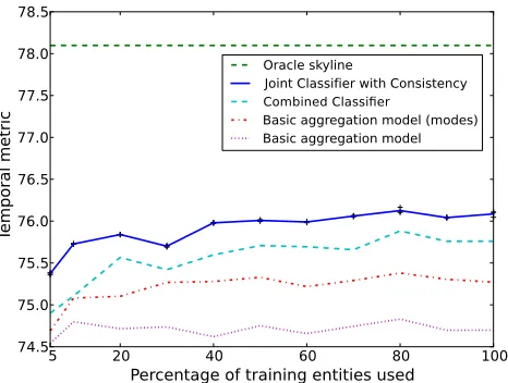
Figure 2: Performance of models and baselines on devel-opment data while varying amount of training data. Not pictured: The null baseline at 58.8%.
of this baseline is primarily to show the approximate minimal value for the temporal metric.
We provide two other baselines to describe heuris-tic methods of aggregating the hard decisions from the classifier functionC learned in§3.2. These are unlike the CC model which uses the soft decisions ofC. Both of these baselines maintain lists of pos-sible starts and ends for each fluent. If the classifier assignsSTART AND END, we add the candidate tem-poral expression to both. The first baseline, basic
aggregation, is along the same lines as the
aggrega-tion method used in Artiles et al. (2011), a state-of-the-art system. Our baseline assigns the earliest start and the latest end as the bounds for each fluent, as-signing ±∞ for empty lists. The second baseline,
basic aggregation (modes), is the same except that it
uses the mode from each list.
To determine the best possible score given our temporal expression retrieval system, we calculate the oracle score by assigning each fluent the span which maximizes the temporal metric. The oracle score can differ from a perfect score since we can only use candidate temporal expressions as values for a fluent if (a) mentions of the fluent are retriev-able in our source documents, (b) the temporal ex-pression mention appears nearby, and (c) our tem-poral expression extractor is able to recognize it cor-rectly. Nevertheless, it is still a reasonable upper bound in our setting.
Model Dev Test
Oracle 78.1 75.2
Joint Classifier with Consistency 76.1 72.2
Combined Classifier 75.8 71.5 Basic aggregation (modes) 75.3 71.2
Basic aggregation 74.7 70.5
[image:7.612.73.306.56.232.2]null baseline 58.8 55.6
Table 2: Performance of systems on development and test divisions. The Joint classifier with Consistency is the av-erage of three runs with negligible variance (σ≈0.02).
4.3 Results
We present the performance of our models, base-lines, and the oracle in Figure 2 while varying the percentage of training entities. The JCC model (76.1% on development with 100% training enti-ties) is consistently the best non-oracle system. Its gains are larger when the amount of training data is low. This is presumably because the classifier suf-fers from insufficient data and the consistency com-ponent is able to learn consistency rules to recover from this. Both the CC and JCC models outperform the basic aggregation models. This shows the value of incorporating all marginal probabilities. On the test set (Table 2), the JCC model performs even bet-ter in comparison to the simple models, despite the test set being clearly more difficult than the develop-ment set. In this case, the JCC achieves a 36% error reduction over the basic aggregation model.9On the official KBP entities, the oracle score is 92%. Since we use a different set of entities, there is a mismatch between our entities and the source documents re-sulting in a lower oracle score. Addressing this is future work.
[image:7.612.316.541.56.154.2]5 Discussion
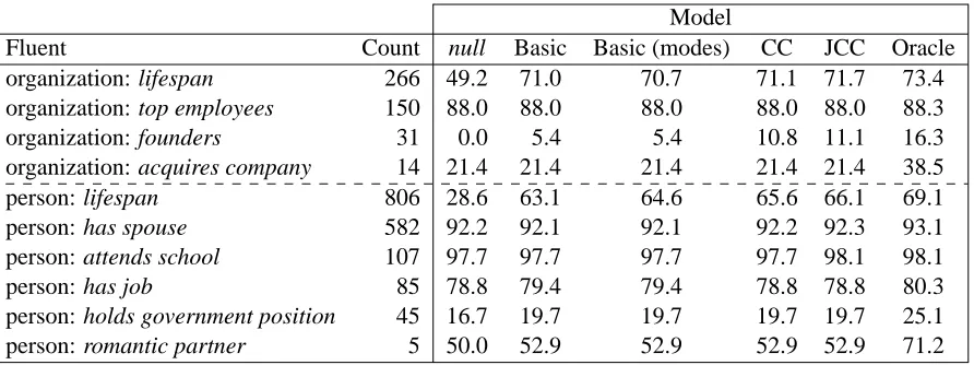
Table 3 shows the performance of four systems and baselines on individual fluent types. The JCC model derives most of its improvement from the two lifespan fluents and other high frequency flu-ents. The lifespan fluents provide the most room for improvement since they tend to contain non-null values a reasonable amount of the time (note how these relations have a large gap between their
ora-9
Model
Fluent Count null Basic Basic (modes) CC JCC Oracle
organization: lifespan 266 49.2 71.0 70.7 71.1 71.7 73.4 organization: top employees 150 88.0 88.0 88.0 88.0 88.0 88.3
organization: founders 31 0.0 5.4 5.4 10.8 11.1 16.3
organization: acquires company 14 21.4 21.4 21.4 21.4 21.4 38.5
person: lifespan 806 28.6 63.1 64.6 65.6 66.1 69.1
person: has spouse 582 92.2 92.1 92.1 92.2 92.3 93.1
person: attends school 107 97.7 97.7 97.7 97.7 98.1 98.1
person: has job 85 78.8 79.4 79.4 78.8 78.8 80.3
[image:8.612.86.532.56.223.2]person: holds government position 45 16.7 19.7 19.7 19.7 19.7 25.1 person: romantic partner 5 50.0 52.9 52.9 52.9 52.9 71.2
Table 3: Fluent-level performance of models and baselines on development data. Scores are calculated with the temporal metric. CC stands for Combined Classifier and JCC for Joint Classifier with Consistency. The JCC model obtains most of its benefits on the two lifespan relations. For attends school, it is the only system able to achieve oracle-level performance. The null baseline is especially strong for several fluents since these tend to be unbounded or (more likely) missing their values in Freebase. The two basic aggregation models differ primarily on their predictions for the lifespan fluents.
cle and null scores). Additionally, the lifespan fluent is always present for entities while other fluents are sparser. For attends school, JCC is the only system able to achieve oracle-level performance. No system improves on the null baseline for acquires company. This is likely due to its sparsity.
Inspecting the multinomials in the consistency component, we can see that the model learns reason-able answers to questions such as whether an entity “was born before getting married?” (yes: 14.8%, no: 0.04%),10“died before their parents were born?” (yes: 0.3%, no: 53.7%) and “finished a job before starting a job (not necessarily the same one)?” (yes: 72.5%, no: 20.5%). Despite some unavoidable noise in the data, it is clear these constraints are useful.
6 Related work
There is a large body of related work that focuses on ordering events or classifying temporal relations between them (Ling and Weld, 2010; Yoshikawa et al., 2009; Chambers and Jurafsky, 2008; Mani et al., 2006, inter alia). Much of this work uses the Allen interval relations (Allen, 1983) which richly describe partial orderings of fluents. We use several of these as fluent-level question templates.
Joint inference has been applied successfully
10
Percentages for “unknown” are omitted here.
to other NLP problems (Roth and Yih, 2004; Toutanova et al., 2008; Martins et al., 2009; Chang et al., 2010; Koo et al., 2010; Berant et al., 2011). Two recent examples in information ex-traction include using Markov Logic for temporal ordering (Ling and Weld, 2010) and using dual-decomposition for event extraction (Riedel and Mc-Callum, 2011).
Our work is closest to Temporal KBP slot filling systems. The CUNY and UNED systems (Artiles et al., 2011; Garrido et al., 2011) for this task used classifiers to determine the relation between tempo-ral expressions and fluents. These systems use the hard decisions from the classifier and combine the decisions by finding a span that includes all temporal expressions. In contrast, our system uses the classi-fier’s marginal probabilities along with the consis-tency component to incorporate global consisconsis-tency constraints. Other participants used rule-based and pattern matching approaches (Byrne and Dunnion, 2011; Surdeanu et al., 2011; Burman et al., 2011).
tempo-ral constraints (e.g., mutual exclusion, containment, and succession) and joint inference. One key dif-ference is that their constraints are included as input rather than learned by the system.
7 Conclusion and future Work
Joint inference can be effectively applied to the task of inferring timelines about named entities. Rather than using hard coded heuristics, our model learns and applies consistency constraints which capture inter-entity and cross-entity rules. Simple inference techniques such as random-restart hillclimbing score well and run efficiently. Both of our models (CC and JCC) obtain a substantial error reductions over sim-pler heuristics-based consistency approaches.
The overall framework can easily be applied to other information extraction tasks. Rather than list-ing rules for consistency, these can be learned and enforced via joint inference. While simple joint in-ference methods such as random-restart hillclimb-ing and Gibbs samplhillclimb-ing worked well in our case, more complex inference methods may be required with more elaborate constraints.
A prime direction for future work is combining our model with a probabilistic relation extraction system. This could be accomplished by using the marginal probabilities on the extracted relations and multiplying them with the probabilities from the classifier and consistency components. Inference would require an additional step which could add or drop candidate fluents. Furthermore, the consistency component can be extended with new question types to incorporate non-temporal constraints as well.
Acknowledgments
The authors would like to thank the Stanford NLP group (with special thanks to Gabor Angeli and Mihai Surdeanu), William Headden, Micha Elsner, Pontus Stenetorp, and our anonymous reviewers for their helpful comments and feedback.
We gratefully acknowledge the support of Defense Advanced Research Projects Agency (DARPA) Machine Reading Program under Air Force Research Laboratory (AFRL) prime contract no. FA8750-09-C-0181. Any opinions, findings, and conclusion or recommendations expressed in this material are those of the author(s) and do not
necessarily reflect the view of the DARPA, AFRL, or the US government.
References
James F. Allen. 1983. Maintaining knowledge about temporal intervals. Communications of the ACM,
26(11):832–843.
Javier Artiles, Qi Li, Taylor Cassidy, Suzanne Tamang, and Heng Ji. 2011. CUNY BLENDER TAC-KBP2011 Temporal Slot Filling System Description. In Proceedings of Text Analysis Conference (TAC), November.
Jonathan Berant, Ido Dagan, and Jacob Goldberger. 2011. Global learning of typed entailment rules. In
Proceedings of the 49th Annual Meeting of the Asso-ciation for Computational Linguistics: Human Lan-guage Technologies, pages 610–619, Portland,
Ore-gon, USA, June. Association for Computational Lin-guistics.
Amev Burman, Arun Jayapal, Sathish Kannan, Madhu Kavilikatta, Ayman Alhelbawy, Leon Derczynski, and Robert Gaizauskas. 2011. USFD at KBP 2011: Entity Linking, Slot Filling and Temporal Bounding. In
Pro-ceedings of Text Analysis Conference (TAC),
Novem-ber.
Lorna Byrne and John Dunnion. 2011. UCD IIRG at TAC 2011. In Proceedings of Text Analysis
Confer-ence (TAC), November.
Nathanael Chambers and Dan Jurafsky. 2008. Jointly combining implicit constraints improves temporal or-dering. In Proceedings of the Conference on
Empir-ical Methods in Natural Language Processing, pages
698–706. Association for Computational Linguistics. Angel X. Chang and Christopher D. Manning. 2012.
SUTIME: A library for recognizing and normalizing time expressions. In 8th International Conference on
Language Resources and Evaluation (LREC 2012),
May.
Ming-Wei Chang, Dan Goldwasser, Dan Roth, and Vivek Srikumar. 2010. Discriminative learning over con-strained latent representations. In Human Language
Technologies: The 2010 Annual Conference of the North American Chapter of the Association for Com-putational Linguistics, pages 429–437. Association for
Computational Linguistics.
Mark Craven and Johan Kumlien. 1999. Constructing biological knowledge bases by extracting information from text sources. In Proceedings of the Seventh
Inter-national Conference on Intelligent Systems for Molec-ular Biology, pages 77–86. Heidelberg, Germany.
on Cross-framework and Cross-domain Parser Evalu-ation.
Jenny R. Finkel, Teg Grenager, and Christopher D. Man-ning. 2005. Incorporating non-local information into information extraction systems by Gibbs sampling. In
Proceedings of the 43rd Annual Meeting on Associ-ation for ComputAssoci-ational Linguistics, pages 363–370.
Association for Computational Linguistics.
Guillermo Garrido, Bernardo Cabaleiro, Anselmo Pe nas, Alvaro Rodrigo, and Damiano Spina. 2011. A distant supervised learning system for the TAC-KBP Slot Fill-ing and Temporal Slot FillFill-ing Tasks. In ProceedFill-ings of
Text Analysis Conference (TAC), November.
Heng Ji, Ralph Grishman, and Hoa Trang Dang. 2011. Overview of the TAC 2011 Knowledge Base Popula-tion track. In Proceedings of Text Analysis Conference
(TAC), November.
Dan Klein and Christopher D. Manning. 2003. Accurate unlexicalized parsing. In Proceedings of the 41st
An-nual Meeting on Association for Computational Lin-guistics, pages 423–430. Association for
Computa-tional Linguistics.
Terry Koo, Alexander M. Rush, Michael Collins, Tommi Jaakkola, and David Sontag. 2010. Dual decompo-sition for parsing with non-projective head automata. In Proceedings of the 2010 Conference on
Empiri-cal Methods in Natural Language Processing, pages
1288–1298. Association for Computational Linguis-tics.
Heeyoung Lee, Yves Peirsman, Angel X. Chang, Nathanael Chambers, Mihai Surdeanu, and Dan Juraf-sky. 2011. Stanford’s Multi-Pass Sieve Coreference Resolution System at the CoNLL-2011 Shared Task. In CoNLL 2011, page 28.
Xiao Ling and Daniel S. Weld. 2010. Temporal infor-mation extraction. In Proceedings of the Twenty Fifth
National Conference on Artificial Intelligence.
Inderjeet Mani, Marc Verhagen, Ben Wellner, Chong Min Lee, and James Pustejovsky. 2006. Machine learning of temporal relations. In Proceedings of the 21st
In-ternational Conference on Computational Linguistics and the 44th Annual Meeting of the Association for Computational Linguistics, pages 753–760.
Associa-tion for ComputaAssocia-tional Linguistics.
Andr´e F. T. Martins, Noah A. Smith, and Eric P. Xing. 2009. Concise integer linear programming formula-tions for dependency parsing. In Proceedings of the
Joint Conference of the 47th Annual Meeting of the ACL and the 4th International Joint Conference on Natural Language Processing of the AFNLP, pages
342–350. Association for Computational Linguistics. Mike Mintz, Steven Bills, Rion Snow, and Dan Jurafsky.
2009. Distant supervision for relation extraction
with-out labeled data. In Proceedings of the Joint
Confer-ence of the 47th Annual Meeting of the ACL and the 4th International Joint Conference on Natural Language Processing of the AFNLP, pages 1003–1011.
Associa-tion for ComputaAssocia-tional Linguistics.
Sebastian Riedel and Andrew McCallum. 2011. Fast and robust joint models for biomedical event extraction. In
Proceedings of the Conference on Empirical Methods in Natural Language Processing (EMNLP ’11), July.
Dan Roth and Wen-tau Yih. 2004. A linear program-ming formulation for global inference in natural lan-guage tasks. In Hwee Tou Ng and Ellen Riloff, editors,
HLT-NAACL 2004 Workshop: Eighth Conference on Computational Natural Language Learning (CoNLL-2004), pages 1–8, Boston, Massachusetts, USA, May
6 - May 7. Association for Computational Linguistics. Mihai Surdeanu, Sonal Gupta, John Bauer, David Mc-Closky, Angel X. Chang, Valentin I. Spitkovsky, and Christopher D. Manning. 2011. Stanford’s Distantly-Supervised Slot-Filling System. In Proceedings of
Text Analysis Conference (TAC), November.
Partha Pratim Talukdar, Derry Wijaya, and Tom Mitchell. 2012. Coupled temporal scoping of relational facts. In
Proceedings of the Fifth ACM International Confer-ence on Web Search and Data Mining, pages 73–82.
ACM.
Kristina Toutanova, Dan Klein, Christopher D. Manning, and Yoram Singer. 2003. Feature-rich part-of-speech tagging with a cyclic dependency network. In
Pro-ceedings of the 2003 Conference of the North Ameri-can Chapter of the Association for Computational Lin-guistics on Human Language Technology, pages 173–
180. Association for Computational Linguistics. Kristina Toutanova, Aria Haghighi, and Christopher D.
Manning. 2008. A global joint model for semantic role labeling. Computational Linguistics, 34(2):161– 191.
Yafang Wang, Bing Yang, Lizhen Qu, Marc Spaniol, and Gerhard Weikum. 2011. Harvesting facts from textual web sources by constrained label propagation. In
Pro-ceedings of the 20th ACM International Conference on Information and Knowledge Management, pages 837–
846. ACM.
Katsumasa Yoshikawa, Sebastian Riedel, Yuji Mat-sumoto, and Masayuki Asahara. 2009. Jointly iden-tifying temporal relations with Markov Logic. In
Pro-ceedings of the Joint Conference of the 47th Annual Meeting of the ACL and the 4th International Joint Conference on Natural Language Processing of the AFNLP, pages 405–413. Association for