Hierarchical Discriminative Classification for Text Based Geolocation

Hierarchical Discriminative Classification for Text-Based Geolocation

Benjamin Wing† _{Jason Baldridge}†

†_{Department of Linguistics, University of Texas at Austin}

[email protected], [email protected]

Abstract

Text-based document geolocation is com-monly rooted in language-based infor-mation retrieval techniques over geodesic grids. These methods ignore the natural hierarchy of cells in such grids and fall afoul of independence assumptions. We demonstrate the effectiveness of using lo-gistic regression models on a hierarchy of nodes in the grid, which improves upon the state of the art accuracy by several percent and reduces mean error distances by hundreds of kilometers on data from Twitter, Wikipedia, and Flickr. We also show that logistic regression performs fea-ture selection effectively, assigning high weights to geocentric terms.

1 Introduction

Document geolocation is the identification of the location—a specific latitude and longitude—that forms the primary focus of a given document. This assumes that a document can be adequately associ-ated with asinglelocation, which is only valid for certain documents, generally of fairly small size. Nonetheless, there are many natural situations in which such collections arise. For example, a great number of articles in Wikipedia have been man-ually geotagged; this allows those articles to ap-pear in their geographic locations in geobrowsers like Google Earth. Images in social networks such as Flickr may be geotagged by a camera and their textual tags can be treated as documents. Like-wise, tweets in Twitter are often geotagged; in this case, it is possible to view either an individual tweet or the collection of tweets for a given user as a document, respectively identifying the loca-tion as the place from which the tweet was sent or the home location of the user.

Early work on document geolocation used heuristic algorithms, predicting locations based on

toponyms in the text (named locations, determined with the aid of a gazetteer) (Ding et al., 2000; Smith and Crane, 2001). More recently, vari-ous researchers have used topic models for doc-ument geolocation (Ahmed et al., 2013; Hong et al., 2012; Eisenstein et al., 2011; Eisenstein et al., 2010) or other types of geographic document summarization (Mehrotra et al., 2013; Adams and Janowicz, 2012; Hao et al., 2010). A number of researchers have used metadata of various sorts for document or user geolocation, including doc-ument links and social network connections. This research has sometimes been applied to Wikipedia (Overell, 2009) or Facebook (Backstrom et al., 2010) but more commonly to Twitter, focusing variously on friends and followers (McGee et al., 2013; Sadilek et al., 2012), time zone (Mahmud et al., 2012), declared location (Hecht et al., 2011), or a combination of these (Schulz et al., 2013).

We tackle document geolocation using super-vised methods based on the textual content of documents, ignoring their metadata. Metadata-based approaches can achieve great accuracy (e.g. Schulz et al. (2013) obtain 79% accuracy within 100 miles for a US-based Twitter corpus, com-pared with 49% using our methods on a compa-rable corpus), but are very specific to the partic-ular corpus and the types of metadata it makes available. For Twitter, the metadata includes the user’s declared location and time zone, infor-mation which greatly simplifies geolocation and which is unavailable for other types of corpora, such as Wikipedia. In many cases essentially no metadata is available at all, as in historical corpora in the digital humanities (Lunenfeld et al., 2012), such as those in the Perseus project (Crane, 2012). Text-based approaches can be applied to all types of corpora; metadata can be additionally incorpo-rated when available (Han and Cook, 2013).

We introduce a hierarchical discriminative clas-sification method for text-based geotagging. We

apply this to corpora in three languages (English, German and Portuguese). This method scales well to large training sets and greatly improves results across a wide variety of corpora, beat-ing current state-of-the-art results by wide mar-gins, including Twitter users (Han et al., 2014, henceforth Han14; Roller et al., 2012, henceforth Roller12); Wikipedia articles (Roller12; Wing and Baldridge, 2011, henceforth WB11); and Flickr images (O’Hare and Murdock, 2013, henceforth OM13). Importantly, this is the first method that improves upon straight uniform-grid Naive Bayes on all of these corpora, in contrast withk-d trees (Roller12) and the current state-of-the-art tech-nique for Twitter users of geographically-salient feature selection (Han14).

We also show, contrary to Han14, that logistic regression when properly optimized is more ac-curate than state-of-the-art techniques, including feature selection, and fast enough to run on large corpora. Logistic regression itself very effectively picks out words with high geographic significance. In addition, because logistic regression does not assume feature independence, complex and over-lapping features of various sorts can be employed.

2 Data

We work with six large datasets: two of geotagged tweets, three of Wikipedia articles, and one of Flickr photos. One of the two Twitter datasets is primarily localized to the United States, while the remaining datasets cover the whole world.

TWUS is a dataset of tweets compiled by

Roller12. A document in this dataset is the con-catenation of all tweets by a single user, as long as at least one of the user’s tweets is geotagged with specific, GPS-assigned latitude/longitude co-ordinates. The earliest such tweet determines the user’s location. Tweets outside of a bounding box covering the contiguous United States (including parts of Canada and Mexico) were discarded, as well as users that may be spammers or robots (based on the number of followers, followees and tweets). The resulting dataset contains 38M tweets from 450K users, of which 10,000 each are re-served for the development and test sets.

TWWORLD is a dataset of tweets compiled by

Han et al. (2012). It was collected in a simi-lar fashion to TWUS but differs in that it covers the entire Earth instead of primarily the United States, and consists only of geotagged tweets.

Non-English tweets and those not near a city were removed, and non-alphabetic, overly short and overly infrequent words were filtered. The result-ing dataset consists of 1.4M users, with 10,000 each reserved for the development and test sets.

ENWIKI13is a dataset consisting of the 864K

geotagged articles (out of 14M articles in all) in the November 4, 2013 English Wikipedia dump. It is comparable to the dataset used in WB11 and was processed using an analogous fashion. The articles were randomly split 80/10/10 into training, development and test sets.

DEWIKI14is a similar dataset consisting of the

324K geotagged articles (out of 1.71M articles in all) in the July 5, 2014 German Wikipedia dump.

PTWIKI14is a similar dataset consisting of the

131K geotagged articles (out of 817K articles in all) in the June 24, 2014 Portuguese Wikipedia dump.

COPHIR (Bolettieri et al., 2009) is a large

dataset of images from the photo-sharing social network Flickr. It consists of 106M images, of which 8.7M are geotagged. Most images contain user-provided tags describing them. We follow al-gorithms described in OM13 in order to make di-rect comparison possible. This involves removing photos with empty tag sets and performing bulk upload filtering, retaining only one of a set of pho-tos from a given user with identical tag sets. The resulting reduced set of 2.8M images is then di-vided 80/10/10 into training, development and test sets. The tag set of each photo is concatenated into a single piece of text (in the process losing user-supplied tag boundary information in the case of multi-word tags).

Our code and processed corpora are available for download.1

3 Supervised models for document geolocation

The dominant approach for text-based geolocation comes from language modeling approaches in in-formation retrieval (Ponte and Croft, 1998; Man-ning et al., 2008). For this general strategy, the Earth is sub-divided into a grid, and then each training set document is associated with the cell that contains it. Some model (typically Naive Bayes) is then used to characterize each cell and

1_{https://github.com/utcompling/}

enable new documents to be assigned a latitude and longitude based on those characterizations. There are several options for constructing the grid and for modeling, which we review next.

3.1 Geodesic grids

The simplest grid is a uniform rectangular one with cells of equal-sized degrees, which was used by Serdyukov et al. (2009) for Flickr images and WB11 for Twitter and Wikipedia. This has two problems. Compared to a grid that takes document density into account, it over-represents rural areas at the expense of urban areas. Furthermore, the rectangles are not equal-area, but shrink in width away from the equator (although the shrinkage is mild until near the poles). Roller12 tackle the for-mer issue by using an adaptive grid based onk-d trees, while Dias et al. (2012) handle the latter is-sue with an equal-area quaternary triangular mesh. An additional issue with geodesic grids is that a single metro area may be divided between two or more cells. This can introduce a statistical bias known as the modifiable areal unit problem (Gehlke and Biehl, 1934; Openshaw, 1983). One way to mitigate this, implemented in Roller12’s code but not investigated in their paper, is to di-vide a cell in a k-d tree in such a way as to pro-duce the maximum margin between the dividing line and the nearest document on each side.

A more direct method is to use a city-based rep-resentation, either with a full set of sufficiently-sized cities covering the Earth and taken from a comprehensive gazetteer (Han14) or a limited, pre-specified set of cities (Kinsella et al., 2011; Sadilek et al., 2012). Han14 amalgamate cities into nearby larger cities within the same state (or equivalent); an even more direct method would use census-tract boundaries when available. Dis-advantages of these methods are the dependency on time-specific population data, making them un-suitable for some corpora (e.g. 19th-century doc-uments); the difficulty in adjusting grid resolution in a principled fashion; and the fact that not all documents are near a city (Han14 find that 8% of tweets are “rural” and cannot predicted by their model).

We construct rectangular grids, since they are very easy to implement and Dias et al. (2012)’s triangular mesh did not yield consistently better results over Wikipedia. We use both uniform grids andk-d tree grids with midpoint splitting.

3.2 Naive Bayes

A geodesic grid of sufficient granularity creates a large decision space, when each cell is viewed as a label to be predicted by some classifier. This situation naturally lends itself to simple, scalable language-modeling approaches. For this general strategy, each cell is characterized by a pseudo-document constructed from the training docu-ments that it contains. A test document’s location is then chosen based on the cell with the most sim-ilar language model according to standard mea-sures such as Kullback-Leibler (KL) divergence (Zhai and Lafferty, 2001), which seeks the cell whose language model is closest to the test doc-ument’s, or Naive Bayes (Lewis, 1998), which chooses the cell that assigns the highest probabil-ity to the test document.

Han14, Roller12 and WB11 follow this strat-egy, using KL divergence in preference to Naive Bayes. However, we find that Naive Bayes in con-junction with Dirichlet smoothing (Smucker and Allan, 2006) works at least as well when appropri-ately tuned. Dirichlet smoothing is a type of dis-counting model that interpolates between the un-smoothed (maximum-likelihood) document distri-bution θ˜di of a document di and the unsmoothed distribution θ˜D over all documents. A general

interpolation model for the smoothed distribution

θdi has the following form:

P(w|θdi) = (1−λdi)P(w|θ˜di) +λdiP(w|θ˜D) (1)

where the discount factorλdiindicates how much probability mass to reserve for unseen words. For Dirichlet smoothing,λdiis set as:

λdi = 1−

|di|

|di|+m (2)

where |di| is the size of the document and m is

a tunable parameter. This has the effect of re-lying more on di’s distribution and less on the

global distribution for larger documents that pro-vide more epro-vidence than shorter ones. Naive Bayes models are estimated easily, which allows them to handle fine-scale grid resolutions with po-tentially thousands or even hundreds of thousands of non-empty cells to choose among.

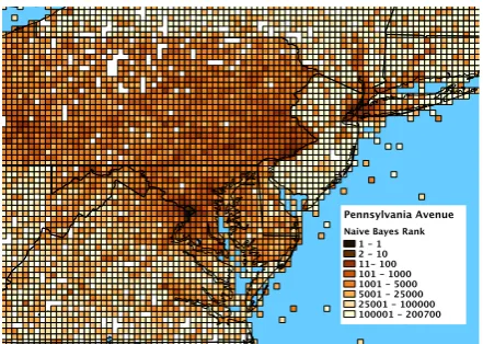
Figure 1: Relative Naive Bayes rank of cells for ENWIKI13 test document Pennsylvania Avenue

(Washington, DC), surrounding the true location.

the test documentPennsylvania Avenue (Washing-ton, DC)in ENWIKI13, for a uniform 0.1◦ grid. The top-ranked cell is the correct one.

3.3 Logistic regression

The use of discrete cells over the Earth’s sur-face allows any classification strategy to be em-ployed, including discriminative classifiers such as logistic regression. Logistic regression often pro-duces propro-duces better results than generative clas-sifiers at the cost of more time-consuming train-ing, which limits the size of the problems it may be applied to. Training is generally unable to scale to encompass several thousand or more distinct la-bels, as is the case with fine-scale grids of the sort we may employ. Nonetheless we find flat logis-tic regression to be effective on most of our large-scale corpora, and the hierarchical classification strategy discussed in §4 allows us to take advan-tage of logistic regression without incurring such a high training cost.

3.4 Feature selection

Naive Bayes assumes that features are indepen-dent, which penalizes models that must accom-modate many features that are poor indicators and which can gang up on the good features. Large improvements have been obtained by reducing the set of words used as features to those that are geographically salient. Cheng et al. (2010; 2013) model word locality using a unimodal dis-tribution taken from Backstrom et al. (2008) and train a classifier to identify geographically lo-cal words based on this distribution. This un-fortunately requires a large hand-annotated

cor-pus for training. Han14 systematically investi-gate various feature selection methods for find-ing geo-indicative words, such as information gain ratio (IGR) (Quinlan, 1993), Ripley’s K statis-tic (O’Sullivan and Unwin, 2010) and geographic density (Chang et al., 2012), showing significant improvements on TWUS and TWWORLD(§2).

For comparison with Han14, we test against an additional baseline: Naive Bayes combined with feature selection done using IGR. Following Han14, we first eliminate words which occur less than 10 times, have non-alphabetic characters in them or are shorter than 3 characters. We then compute the IGR for the remaining words across all cells at a given cell size or bucket size, select the topN%for somecutoff percentageN (which we vary in increments of 2%), and then run Naive Bayes at the same cell size or bucket size.

4 Hierarchical classification

To overcome the limitations of discriminative clas-sifiers in terms of the maximum number of cells they can handle, we introduce hierarchical classifi-cation (Silla Jr. and Freitas, 2011) for geoloclassifi-cation. Dias et al. (2012) use a simple two-level genera-tive hierarchical approach using Naive Bayes, but to our knowledge no previous work implements a multi-level discriminative hierarchical model with beam search for geolocation.

To construct the hierarchy, we start with a root cellcrootthat spans the entire Earth and from there

build a tree of cells at different scales, from coarse to fine. A cell at a given level is subdivided to create smaller cells at the next level of resolution that altogether cover the same area as their parent. We use thelocal classifier per parentapproach to hierarchical classification (Silla Jr. and Fre-itas, 2011) in which an independent classifier is learned for every node of the hierarchy above the leaf nodes. The probability of any node in the hi-erarchy is the product of the probabilities of that node and all of its ancestors, up to the root. This is defined recursively as:

P(croot) = 1.0

P(cj) = P(cj|↑cj)P(↑cj) (3)

where↑cj indicatescj’s parent in the hierarchy.

probability of every leaf cell using equation 3, we use a stratified beam search: starting at the root cell, keep the b highest-probability cells at each level until reaching the leaf node level. With a tight beam—which we show to be very effective— this dramatically reduces the number of model evaluations that must be performed at test time.

Grid size parameters Two factors determine the size of the grids at each level. The first-level grid is constructed the same as for Naive Bayes or flat logistic regression and is controlled by its own parameter. In addition, thesubdivision factor

N determines how we subdivide each cell to get from one level to the next. Both factors must be optimized appropriately.

For the uniform grid, we subdivide each cell intoNxNsubcells. In practice, there may actually be fewer subcells, because some of the potential subcells may be empty (contain no documents).

For the k-d grid, if level 1 is created using a bucket sizeB (i.e. we recursively divide cells as long as their size exceedsB), then level 2 is cre-ated by continuing to recursively divide cells that exceed a smaller bucket sizeB/N. At this point, the subcells of a given level-1 cell are the leaf cells contained with the cell’s geographic area. The construction of level 3 proceeds similarly using bucket sizeB/N2_{, etc.}

Note that the subdivision factor has a different meaning for uniform and k-d tree grids. Further-more, because creating the subdividing cells for a given cell involves dividing byN2_{for the uniform}

grid butN for thek-d tree grid, greater subdivi-sion factors are generally required for thek-d tree grid to achieve similar-scale resolution.

Figure 2 shows the behavior of hierarchical LR using k-d trees for the test document Pennsylva-nia Avenue (Washington, DC)in ENWIKI13. Af-ter ranking the first level, the beam zooms in on the top-ranked cells and constructs a finerk-d tree under each one (one such subtree is shown in the top-right map callout).

5 Experimental Setup

Configurations. We experiment with several methods for configuring the grid and selecting the best cell. For grids, we use either a uniform or

k-dtree grid. For uniform grids, the main tunable parameter is grid size (in degrees), while fork-d trees it is bucket size (BK), i.e. the number of doc-uments above which a node is divided in two.

Figure 2: Relative hierarchical LR rank of cells for ENWIKI13 test document Pennsylvania

Av-enue (Washington, DC), surrounding the true lo-cation. The first callout simply expands a portion of level 1, while the second callout shows a level 1 cell subdivided down to level 2.

For cell choice, the options are:

• NB: Naive Bayes baseline

• IGR: Naive Bayes using features selected by information gain ratio

• FlatLR: logistic regression model over all leaf nodes

• HierLR: product of logistic regression mod-els at each node in a hierarchical grid (eq. 3) For Dirichlet smoothing in conjunction with Naive Bayes, we set the Dirichlet parameter m = 1,000,000, which we found worked well in pre-liminary experiments. For hierarchical classifica-tion, there are additional parameters: subdivision factor (SF) and beam size (BM) (§4), and hierar-chy depth (D) (§6.4). All of our test-set results use a depth of three levels.

Due to its speed and flexibility, we use Vowpal Wabbit (Agarwal et al., 2014) for logistic regres-sion, estimating parameters with limited-memory BFGS (Nocedal, 1980; Byrd et al., 1995). Unless otherwise mentioned, we use 26-bit feature hash-ing (Weinberger et al., 2009) and 40 passes over the data (optimized based on early experiments on development data) and turn off the hold-out mech-anism. For the subcell classifiers in hierarchical classification, which have fewer classes and much less data, we use 24-bit features and 12 passes.

al., 2010) andaccuracy at 161 km(acc@161), i.e. within a 161-km radius, which was introduced by Cheng et al. (2010) as a proxy for accuracy within a metro area. All of these metrics are indepen-dent of cell size, unlike the measure of cell accu-racy (fraction of cells correctly predicted) used in Serdyukov et al. (2009). Following Han14, we use acc@161 on development sets when choosing al-gorithmic parameter values such as cell and bucket sizes.

6 Results 6.1 Twitter

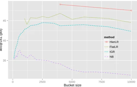
We show the effect of varying cell size in Table 1 andk-d tree bucket size in Figure 3. The number of non-empty cells is shown for each cell size and bucket size. For NB, this is the number of cells against which a comparison must be made for each test document; for FlatLR, this is the number of classes that must be distinguished. For HierLR, no figure is given because it varies from level to level and from classifier to classifier. For example, with a uniform grid and subdivision factor of 3, each level-2 subclassifier will have between 1 and 9 la-bels to choose among, depending on which cells are empty.

Method _{(Deg) (km)}Cell Size #Class _@161Acc. Mean Med._{(km) (km)}

NB 0.17_0.50◦◦ 11,671_2,838 36.6 929.5 496.4_{35.4 889.3 466.6} IGR,CU90% 1.5◦ _{501 45.9 787.5 255.6}

FlatLR

5◦ _{556 59 35.4 727.8 248.7} 4◦ _{445 99 44.4 718.8 227.9} 3◦ _{334 159 47.3 721.3 186.2} 2.5◦ _{278 208 47.5 743.9 198.9} 2◦ _{223 316 46.9 737.7 209.9} 1.5◦ _{167 501 46.6 762.6 226.9} 1◦ _{111 975 43.0 810.0 303.7} HierLR,D2, SF2, BM5 4◦ _{– – 48.6 695.2 182.2} HierLR,D2, SF2, BM2 3◦ _{– – 49.0 725.1 174.6} HierLR,D3, SF2, BM2 3◦ _{– – 49.0 718.9 173.8} HierLR,D2, SF2, BM5 2.5◦ _{– – 48.2 740.9 187.7}

Table 1: Dev set performance for TWUS, with uniform grids. HierLR and IGR parameters op-timized using acc@161. Best metric numbers for a given method are underlined, except that overall best numbers are in bold.

FlatLR does much better than NB and IGR, and HierLR is still better. This is despite logistic re-gression needing to operate at a much lower res-olution.2 _{Interestingly, uniform-grid 2-level} Hi-erLR does better at 4◦ _{with a subdivision factor} 2_{The limiting factor for resolution for us was the 24-hour} per job limit on our computing cluster.

●

●

35 40 45

0 2500 5000 7500 10000

Bucket size

acc@161 (pct)

method

● HierLR FlatLR IGR NB

Figure 3: Dev set performance for TWUS, with

k-d tree grids.

of 2 than the equivalent FlatLR run at 2◦_.

Table 2 shows the test set results for the vari-ous methods and metrics described in§5, on both TWUS and TWWORLD.3 HierLR is the best across all metrics; the best acc@161km and me-dian error is obtained with a uniform grid, while HierLR withk-d trees obtains the best mean error. Compared with vanilla NB, our implementa-tion of NB using IGR feature selecimplementa-tion obtains large gains for TWUS and moderate gains for TWWORLD, showing that IGR can be an effec-tive geolocation method for Twitter. This agrees in general with Han14’s findings. We can only compare our figures directly with Han14 for k-d trees—in this case they use a version of the same software we use and report figures within 1% of ours for TWUS. Their remaining results are com-puted using a city-based grid and an NB imple-mentation with add-one smoothing, and are signif-icantly worse than our uniform-grid NB and IGR figures using Dirichlet smoothing, which is known to significantly outperform add-one smoothing (Smucker and Allan, 2006). For example, for NB they report 30.8% acc@161 for TWUS and 20.0% for TWWORLD, compared with our 36.2% and 30.2% respectively. We suspect an additional rea-son for the discrepancy is due to the limitations of their city-based grid, which has no tunable param-eter to optimize the grid size and requires that test instances not near a city be reported as incorrect.

Our NB figures also beat the KL divergence fig-ures reported in Roller12 for TWUS (which they term UTGEO2011), perhaps again due to the

Corpus TWUS TWWORLD

Method Parameters A@161 Mean Med. Parameters A@161 Mean Med.

NB Uniform 0.17◦ _{36.2 913.8 476.3 1}◦ _{30.2 1690.0 537.2}

NBk-d BK1500 36.2 861.4 444.2 BK500 28.7 1735.0 566.2

IGR Uniform 1.5◦_{,CU90% 46.1 770.3 233.9 1}◦_{,CU90% 31.0 2204.8 574.7}

IGRk-d BK2500, CU90% 44.6 792.0 268.6 BK250, CU92% 29.4 2369.6 655.0

FlatLR Uniform 2.5◦ _{47.2 727.3 195.4 3.7}◦ _{32.1 1736.3 500.0}

FlatLRk-d BK4000 47.4 692.2 197.0 BK12000 27.8 1939.5 651.6

HierLR Uniform 3◦_{,SF2, BM2 49.2 703.6 170.5 5}◦_{,SF2, BM1 32.7 1714.6 490.0}

HierLRk-d BK4000, SF3, BM1 48.0 686.6 191.4 BK60000, SF5, BM1 31.3 1669.6 509.1

Table 2: Performance on the test sets of TWUS and TWWORLDfor different methods and metrics.

ference in smoothing methods.

6.2 Wikipedia

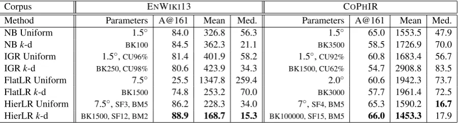
Table 3 shows results on the test set of ENWIKI13 for various methods. Table 5 shows the corre-sponding results for DEWIKI14 and PTWIKI14. In all cases, the best parameters for each method were determined using acc@161 on the develop-ment set, as above.

● ● ● ● ● ● ● ● ● ●●●

● ●●●●●●

● ●

● ●

● ●

●

●

82 84 86 88

0 50 100 150 200 250

K−d subdivision factor

Acc@161 (pct)

beam size

● 1 2 Naive Bayes

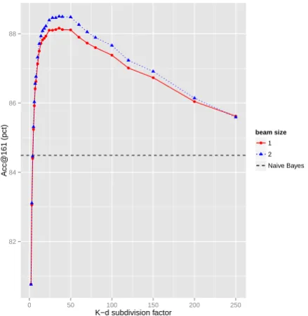
Figure 4: Plot of subdivision factor vs. acc@161 for the ENWIKI13 dev set with 2-level k-d tree HierLR, bucket size 1500. Beam sizes above 2 yield little improvement.

HierLR is clearly the stand-out winner among all methods and metrics, and particularly so for the k-d tree grid. This is achieved through a high sub-division factor, especially in a 2-level hierarchy, where a factor of 36 is best, as shown in Figure 4 for ENWIKI13. (For a 3-level hierarchy, the best subdivision factor is 12.)

Unlike for TWUS, FlatLR simply cannot

com-Method Param #Class A@161 Med. Runtime FlatLR

Uniform

10◦ _{648 19.2 314.1 11h}

8.5◦ _{784 26.5 248.5 16h}

7.5◦ _{933 30.1 232.0 19h}

FlatLR

k-d

BK5000 257 57.1 133.5 5h

BK2500 501 67.5 94.9 9h

BK1500 825 74.7 69.9 16h

HierLR Uniform 7.5

◦_{,SF2,BM1 — 85.2 67.8 23h}

7.5◦_{,SF3,BM5 — 86.1 34.2 27h}

HierLR

k-d

BK1500,SF5,BM1 — 88.2 19.6 23h

BK5000,SF10,BM5 — 88.4 18.3 14h

BK1500,SF12,BM2 — 88.8 15.3 33h

Table 4: Performance/runtime for FlatLR and 3-level HierLR on the ENWIKI13 dev set, with vary-ing parameters.

pete with NB in the larger Wikipedias (ENWIKI13 and DEWIKI14). ENWIKI13 especially has dense coverage across the entire world, whereas TWUS only covers the United States and parts of Canada and Mexico. Thus, there are a much larger num-ber of non-empty cells at a given resolution and much coarser resolution required, especially with the uniform grid. For example, at 7.5◦ _{there are} 933 non-empty cells, comparable to 1◦_{for TWUS.} Table 4 shows the number of classes and runtime for FlatLR and HierLR at different parameter val-ues. The hierarchical classification approach is clearly essential for allowing us to scale the dis-criminative approach for a large, dense dataset across the whole world.

Moving from larger to smaller Wikipedias, FlatLR becomes more competitive. In particular, FlatLR outperforms NB and is close to HierLR for PTWIKI14, the smallest of the three (and signifi-cantly smaller than TWUS). In this case, the rel-atively small size of the dataset and its greater ge-ographic specificity (many articles are located in Brazil or Portugal) allows for a fine enough reso-lution to make FlatLR perform well—comparable to or even finer than NB.

Corpus ENWIKI13 COPHIR

Method Parameters A@161 Mean Med. Parameters A@161 Mean Med.

NB Uniform 1.5◦ _{84.0 326.8 56.3 1.5}◦ _{65.0 1553.5 47.9}

NBk-d BK100 84.5 362.3 21.1 BK3500 58.5 1726.9 70.0

IGR Uniform 1.5◦_{,CU96% 81.4 401.9 58.2 1.5}◦_{,CU92% 60.8 1683.4 56.7}

IGRk-d BK250, CU98% 80.6 423.9 34.3 BK1500, CU62% 54.7 2908.8 83.5

FlatLR Uniform 7.5◦ _{25.5 1347.8 259.4 2.0}◦ _{60.6 1942.3 73.7}

FlatLRk-d BK1500 74.8 253.2 70.0 BK3000 57.7 1961.4 72.5

HierLR Uniform 7.5◦_{,SF3, BM5 86.2 228.3 34.0 7}◦_{,SF4, BM5 65.3 1590.2 16.7}

HierLRk-d BK1500, SF12, BM2 88.9 168.7 15.3 BK100000, SF15, BM5 66.0 1453.3 17.9

Table 3: Performance on the test sets of ENWIKI13 and COPHIR for different methods and metrics.

NB uniform, and HierLR outperforms both, but by greatly varying amounts, with only a 1% differ-ence for DEWIKI14 but 12% for PTWIKI14. It’s unclear what causes these variations, although it’s worth noting that Roller12’s NBk-d figures on an older English Wikipedia corpus were are notice-ably higher than our figures: They report 90.3% acc@161, compared with our 84.5%. We verified that this is due to corpus differences: we obtain their performance when we run on their Wikipedia corpus. This suggests that the various differences may be due to vagaries of the individual corpora, e.g. the presence of differing numbers of geo-tagged stub articles, which are very short and thus hard to geolocate.

As for IGR, though it is competitive for Twitter, it performs badly here—in fact, it is even worse than plain Naive Bayes for all three Wikipedias (likewise for COPHIR, in the next section).

6.3 CoPhIR

Table 3 shows results on the test set of COPHIR for various methods, similarly to the ENWIKI13 results. HierLR is again the clear winner. Unlike for ENWIKI13, FlatLR is able to do fairly well. IGR performs poorly, especially when combined withk-d.

In general, as can be seen, for COPHIR the median figures are very low but the mean figures very high, meaning there are many images that can be very accurately placed while the remainder are very difficult to place. (The former images likely have the location mentioned in the tags, while the latter do not.)

For COPHIR, and also TWWORLD, HierLR performs best when the root level is significantly coarser than the cell or bucket size that is best for FlatLR. The best setting for the root level appears to be correlated with cell accuracy, which in gen-eral increases with larger cell sizes. The intuition

here is that HierLR works by drilling down from a single top-level child of the root cell. Thus, the higher the cell accuracy, the greater the fraction of test instances that can be improved in this fash-ion, and in general the better the ultimate values of the main metrics. (The above discussion isn’t strictly true for beam sizes above 1, but these tend to produce marginal improvements, with little if any gain from going above a beam size of 5.) The large size of a coarse root-child cell, and corre-spondingly poor results for acc@161, can be off-set by a high subdivision factor, which does not materially slow down the training process.

Our NB results are not directly comparable with OM13’s results on COPHIR because they use var-ious cell-based accuracy metrics while we use cell-size-independent metrics. The closest to our acc@161 metric is their Ac1 metric, which at a cell size of 100 km corresponds to a 300km-per-side square at the equator, roughly comparable to our 161-km-radius circle. They report Ac1 figures of 57.7% for term frequency and 65.3% for user frequency, which counts the number of distinct users in a cell using a given term and is intended to offset bias resulting from users who upload a large batch of similar photos at a given location. Our term frequency figure of 65.0% significantly beats theirs, but we found that user frequency actually degraded our dev set results by 5%. The reason for this discrepancy is unclear.

6.4 Parameterization variations

Corpus DEWIKI14 PTWIKI14

Method Parameters A@161 Mean Med. Parameters A@161 Mean Med.

NB Uniform 1◦ _{88.4 257.9 35.0 1}◦ _{76.6 470.0 48.3}

NBk-d BK25 89.3 192.0 7.6 BK100 77.1 325.0 45.9

IGR Uniform 2◦_{,CU82% 87.1 312.9 68.2 2}◦_{,CU54% 71.3 594.6 89.4}

IGRk-d BK50, CU100% 86.0 226.8 10.9 BK100, CU100% 71.3 491.9 57.7

FlatLR Uniform 5◦ _{55.1 340.4 150.1 2}◦ _{88.9 320.0 70.8}

FlatLRk-d BK350 82.0 193.2 24.5 BK25 86.8 320.8 30.0

HierLR Uniform 7◦_{,SF3, BM5 88.5 184.8 30.0 7}◦_{,SF2, BM5 88.6 223.5 64.7}

HierLRk-d BK3500, SF25, BM5 90.2 122.5 8.6 BK250, SF12, BM2 89.5 186.6 27.2

Table 5: Performance on the test sets of DEWIKI14 and PTWIKI14 for different methods and metrics.

dev set, the “best” uniform NB parameter of1.5◦_, as optimized on acc@161, yields a median error of 56.1 km, but an error of just 16.7 km can be achieved with the parameter setting0.25◦ _(which, however, drops acc@161 from 83.8% to 78.3% in the process). Similarly, for the COPHIR dev set, the optimized uniform 2-level HierLR median error of 46.6 km can be reduced to just 8.1 km by dropping from7◦ _to3.5◦ _{and bumping up the} subdivision factor from 4 to 35—again, causing a drop in acc@161 from 68.6% to 65.5%.

Hierarchy depth. We use a 3-level hierarchy throughout for the test set results. Evaluation on development data showed that 2-level hierarchies perform comparably for several data sets, but are less effective overall. We did not find improve-ments from using more than three levels. When using a simple local classifier per parent approach as we do, which chains together spines of related but independently trained classifiers when assign-ing a probability to a leaf cell, most of the ben-efit presumably comes from simply enabling lo-gistic regression to be used with fine-grained leaf cells, overcoming the limitations of FlatLR. Fur-ther benefits of the hierarchical approach might be achieved with the data-biasing and bottom-up er-ror propagation techniques of Bennett and Nguyen (2009) or the hierarchical Bayesian approach of Gopal et al. (2012), which is able to handle large-scale corpora and thousands of classes.

6.5 Feature Selection

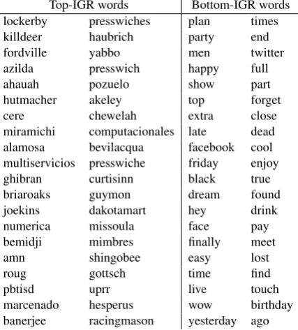
The main focus of Han14 is identifying geograph-ically salient words through feature selection. Lo-gistic regression performs feature selection natu-rally by assigning higher weights to features that better discriminate among the target classes.

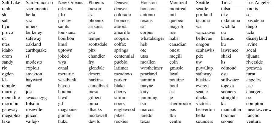
Table 6 shows the top 20 features ranked by fea-ture weight for a number of different cells, labeled

by the largest city in the cell. The features were produced using a uniform 5◦ _{grid, trained using} 27-bit features and 40 passes over TWUS. The high number of bits per feature were chosen to en-sure as few collisions as possible of different fea-tures (as it would be impossible to distinguish two words that were hashed together).

Most words are clearly region specific, con-sisting of cities, states and abbreviations, sports teams (broncos, texans, niners, saints), well-known streets (bourbon, folsom), characteristic features (desert,bayou,earthquake,temple), local brands (whataburger, soopers, heb), local foods (gumbo,poutine), and dialect terms (hella,buku).

Top-IGR words Bottom-IGR words lockerby presswiches plan times

killdeer haubrich party end

fordville yabbo men twitter

azilda presswich happy full

ahauah pozuelo show part

hutmacher akeley top forget

cere chewelah extra close

miramichi computacionales late dead alamosa bevilacqua facebook cool multiservicios presswiche friday enjoy ghibran curtisinn black true

briaroaks guymon dream found

joekins dakotamart hey drink

numerica missoula face pay

bemidji mimbres finally meet

amn shingobee easy lost

roug gottsch time find

pbtisd uprr live touch

marcenado hesperus wow birthday banerjee racingmason yesterday ago Table 7: Top and bottom 40 features selected using IGR for TWUS with a uniform 1.5◦grid.

Salt Lake San Francisco New Orleans Phoenix Denver Houston Montreal Seattle Tulsa Los Angeles utah sacramento orleans tucson denver houston montreal seattle tulsa knotts slc hella jtfo az colorado antonio mtl portland okc sd salt sac prelaw phoenix broncos texans quebec tacoma oklahoma pasadena byu niners saints arizona aurora sa magrib wa wichita diego provo berkeley louisiana asu amarillo corpus rue vancouver ou ucla ut safeway bourbon tempe soopers whataburger habs bellevue kansas disneyland utes oakland kmsl scottsdale colfax heb canadian oregon ku irvine idaho earthquake uptown phx springs otc ouest seahawks lawrence socal orem sf joked chandler centennial utsa mcgill pdx shaki tijuana sandy modesto wya fry pueblo mcallen coin uw ks riverside rio exploit canal glendale larimer westheimer gmusic puyallup edmond pomona ogden stockton metairie desert meadows pearland laval safeway osu turnt lds hayward westbank harkins parker jammin poutine huskies stillwater angeles temple cal bayou camelback blake mayne boul everett topeka usc murray jose houma mesa cherry katy est seatac sooners chargers menudito swaaaaggg lawd gilbert siiiiim jamming je ducks straighht oc mormon folsom gtf pima coors tsu sherbrooke victoria kc compton gateway roseville magazine dbacks englewood marcos pas beaverton manhattan meadowview megaplex juiced gumbo mcdowell pikes laredo fkn hella boomer rancho lake vallejo buku devils rockies texas centre sounders sooner ventura

Table 6: Top 20 features selected for various regions using logistic regression on TWUS with a uniform 5◦_grid.

which have geographic significance, while the bot-tom words are quite common. To some extent this is a feature of IGR, since it divides by the binary entropy of each word, which is directly related to its frequency. However, it shows why cutoffs around 90% of the original feature set are neces-sary to achieve good performance on the Twitter corpora. (IGR does not perform well on Wikipedia or COPHIR, as shown above.)

7 Conclusion

This paper demonstrates that major performance improvements to geolocation based only on text can be obtained by using a hierarchy of logistic regression classifiers. Logistic regression also al-lows for the use of complex, interdependent fea-tures, beyond the simple unigram models com-monly employed. Our preliminary experiments did not show noticeable improvements from bi-gram or character-based features, but it is pos-sible that higher-level features such as morpho-logical, part-of-speech or syntactic features could yield further performance gains. And, of course, these improved text-based models may help de-crease error even further when metadata (e.g. time zone and declared location) are available.

An interesting extension of this work is to rely upon the natural clustering of related documents. Joint modeling of geographic topics and loca-tions has been attempted (see§1), but has gener-ally been applied to much smaller corpora than those considered here. Skiles (2012) found

sig-nificant improvements by clustering the training documents of large-scale corpora using K-means, training separate models from each cluster, and es-timating a test document’s location with the clus-ter model returning the best overall similarity (e.g. through KL divergence). Bergsma et al. (2013) likewise cluster tweets using K-means but predict location only at the country level. Such methods could be combined with hierarchical classification to yield further gains.

Acknowledgments

We would like to thank Grant Delozier for as-sistance in generating choropleth graphs, and the three anonymous reviewers for their feedback. This research was supported by a grant from the Morris Memorial Trust Fund of the New York Community Trust.

References

Benjamin Adams and Krzysztof Janowicz. 2012. On the geo-indicativeness of non-georeferenced text. In John G. Breslin, Nicole B. Ellison, James G. Shana-han, and Zeynep Tufekci, editors,ICWSM’12: Pro-ceedings of the 6th International AAAI Conference

on Weblogs and Social Media. The AAAI Press.

Alekh Agarwal, Oliveier Chapelle, Miroslav Dud´ık, and John Langford. 2014. A reliable effective teras-cale linear learning system. Journal of Machine

Learning Research, 15:1111–1133.

locations from social media posts. InProceedings of the 22nd International Conference on World Wide Web, WWW ’13, pages 25–36, Republic and Canton of Geneva, Switzerland. International World Wide Web Conferences Steering Committee.

Lars Backstrom, Jon Kleinberg, Ravi Kumar, and Jas-mine Novak. 2008. Spatial variation in search en-gine queries. In Proceedings of the 17th

Interna-tional Conference on World Wide Web, WWW ’08,

pages 357–366, New York, NY, USA. ACM. Lars Backstrom, Eric Sun, and Cameron Marlow.

2010. Find me if you can: improving geographi-cal prediction with social and spatial proximity. In Proceedings of the 19th international conference on

World wide web, WWW ’10, pages 61–70, New

York, NY, USA. ACM.

Paul N. Bennett and Nam Nguyen. 2009. Refined ex-perts: improving classification in large taxonomies. In James Allan, Javed A. Aslam, Mark Sanderson, ChengXiang Zhai, and Justin Zobel, editors,SIGIR, pages 11–18. ACM.

Shane Bergsma, Mark Dredze, Benjamin Van Durme, Theresa Wilson, and David Yarowsky. 2013. Broadly improving user classification via communication-based name and location clus-tering on twitter. In Proceedings of the 2013 Conference of the North American Chapter of the Association for Computational Linguistics: Human

Language Technologies, pages 1010–1019, Atlanta,

Georgia, June. Association for Computational Linguistics.

Paolo Bolettieri, Andrea Esuli, Fabrizio Falchi, Clau-dio Lucchese, Raffaele Perego, Tommaso Piccioli, and Fausto Rabitti. 2009. Cophir: a test col-lection for content-based image retrieval. CoRR, abs/0905.4627.

Richard H Byrd, Peihuang Lu, Jorge Nocedal, and Ciyou Zhu. 1995. A limited memory algorithm for bound constrained optimization. SIAM Journal on Scientific Computing, 16(5):1190–1208.

Hau-Wen Chang, Dongwon Lee, Mohammed Eltaher, and Jeongkyu Lee. 2012. @phillies tweeting from philly? predicting twitter user locations with spatial word usage. In Proceedings of the 2012 Interna-tional Conference on Advances in Social Networks

Analysis and Mining (ASONAM 2012), pages 111–

118. IEEE Computer Society.

Zhiyuan Cheng, James Caverlee, and Kyumin Lee. 2010. You are where you tweet: A content-based ap-proach to geo-locating twitter users. InProceedings of the 19th ACM International Conference on

In-formation and Knowledge Management, pages 759–

768.

Zhiyuan Cheng, James Caverlee, and Kyumin Lee. 2013. A content-driven framework for geolocating microblog users. ACM Trans. Intell. Syst. Technol., 4(1):2:1–2:27, February.

Gregory Crane, 2012. The Perseus Project, pages 644– 653. SAGE Publications, Inc.

Duarte Dias, Ivo Anast´acio, and Bruno Martins. 2012. A Language Modeling Approach for Georeferenc-ing Textual Documents. InProceedings of the Span-ish Conference in Information Retrieval.

Junyan Ding, Luis Gravano, and Narayanan Shivaku-mar. 2000. Computing geographical scopes of web resources. InProceedings of the 26th International

Conference on Very Large Data Bases, VLDB ’00,

pages 545–556, San Francisco, CA, USA. Morgan Kaufmann Publishers Inc.

Jacob Eisenstein, Brendan O’Connor, Noah A. Smith, and Eric P. Xing. 2010. A latent variable model for geographic lexical variation. In Proceedings of the 2010 Conference on Empirical Methods in

Natural Language Processing, pages 1277–1287,

Cambridge, MA, October. Association for Compu-tational Linguistics.

Jacon Eisenstein, Ahmed Ahmed, and Eric P. Xing. 2011. Sparse additive generative models of text. In Proceedings of the 28th International Conference on

Machine Learning, pages 1041–1048.

Charles E. Gehlke and Katherine Biehl. 1934. Certain effects of grouping upon the size of the correlation coefficient in census tract material. Journal of the American Statistical Association, 29(185):169–170. Siddharth Gopal, Yiming Yang, Bing Bai, and Alexan-dru Niculescu-Mizil. 2012. Bayesian models for large-scale hierarchical classification. In Peter L. Bartlett, Fernando C. N. Pereira, Christopher J. C. Burges, Lon Bottou, and Kilian Q. Weinberger, edi-tors,NIPS, pages 2420–2428.

Bo Han and Paul Cook. 2013. A stacking-based ap-proach to twitter user geolocation prediction. InIn Proceedings of the 51st Annual Meeting of the Asso-ciation for Computational Linguistics (ACL 2013):

System Demonstrations, pages 7–12.

Bo Han, Paul Cook, and Tim Baldwin. 2012. Geotion predicGeotion in social media data by finding loca-tion indicative words. InInternational Conference

on Computational Linguistics (COLING), page 17,

Mumbai, India, December.

Bo Han, Paul Cook, and Tim Baldwin. 2014. Text-based twitter user geolocation prediction. Journal of Artificial Intelligence Research, 49(1):451–500. Qiang Hao, Rui Cai, Changhu Wang, Rong Xiao,

Jiang-Ming Yang, Yanwei Pang, and Lei Zhang. 2010. Equip tourists with knowledge mined from travelogues. In Proceedings of the 19th

interna-tional conference on World wide web, WWW ’10,

pages 401–410, New York, NY, USA. ACM. Brent Hecht, Lichan Hong, Bongwon Suh, and Ed H.

Proceedings of the SIGCHI Conference on Human

Factors in Computing Systems, CHI ’11, pages 237–

246, New York, NY, USA. ACM.

Liangjie Hong, Amr Ahmed, Siva Gurumurthy, Alexander J. Smola, and Kostas Tsioutsiouliklis. 2012. Discovering geographical topics in the twit-ter stream. InProceedings of the 21st International

Conference on World Wide Web, WWW ’12, pages

769–778, New York, NY, USA. ACM.

Sheila Kinsella, Vanessa Murdock, and Neil O’Hare. 2011. “I’m eating a sandwich in Glasgow”: Mod-eling locations with tweets. In Proceedings of the 3rd International Workshop on Search and Mining

User-generated Contents, pages 61–68.

David D. Lewis. 1998. Naive (bayes) at forty: The in-dependence assumption in information retrieval. In Proceedings of the 10th European Conference on

Machine Learning, ECML ’98, pages 4–15,

Lon-don, UK, UK. Springer-Verlag.

Peter Lunenfeld, Anne Burdick, Johanna Drucker, Todd Presner, and Jeffrey Schnapp. 2012. Digital

humanities. MIT Press, Cambridge, MA.

Jalal Mahmud, Jeffrey Nichols, and Clemens Drews. 2012. Where is this tweet from? inferring home locations of twitter users. In John G. Breslin, Nicole B. Ellison, James G. Shanahan, and Zeynep Tufekci, editors,ICWSM’12: Proceedings of the 6th International AAAI Conference on Weblogs and

So-cial Media. The AAAI Press.

Christopher D. Manning, Prabhakar Raghavan, and Hinrich Sch¨utze. 2008. Introduction to Information

Retrieval. Cambridge University Press, Cambridge,

UK.

Jeffrey McGee, James Caverlee, and Zhiyuan Cheng. 2013. Location prediction in social media based on tie strength. In Proceedings of the 22nd ACM In-ternational Conference on Conference on

Informa-tion and Knowledge Management, CIKM ’13, pages

459–468, New York, NY, USA. ACM.

Rishabh Mehrotra, Scott Sanner, Wray Buntine, and Lexing Xie. 2013. Improving lda topic models for microblogs via tweet pooling and automatic label-ing. InProceedings of the 36th International ACM SIGIR Conference on Research and Development in

Information Retrieval, SIGIR ’13, pages 889–892,

New York, NY, USA. ACM.

Jorge Nocedal. 1980. Updating Quasi-Newton Matri-ces with Limited Storage. Mathematics of Compu-tation, 35(151):773–782.

Neil O’Hare and Vanessa Murdock. 2013. Modeling locations with social media. Information Retrieval, 16(1):30–62.

Stan Openshaw. 1983.The modifiable areal unit prob-lem. Geo Books.

David O’Sullivan and David J. Unwin, 2010. Point

Pattern Analysis, pages 121–155. John Wiley &

Sons, Inc.

Simon Overell. 2009. Geographic Information Re-trieval: Classification, Disambiguation and Mod-elling. Ph.D. thesis, Imperial College London. Jay M. Ponte and W. Bruce Croft. 1998. A language

modeling approach to information retrieval. In Pro-ceedings of the 21st annual international ACM SI-GIR conference on Research and development in

information retrieval, SIGIR ’98, pages 275–281,

New York, NY, USA. ACM.

J. Ross Quinlan. 1993. C4.5: Programs for Machine

Learning. Morgan Kaufmann Publishers Inc., San

Francisco, CA, USA.

Stephen Roller, Michael Speriosu, Sarat Rallapalli, Benjamin Wing, and Jason Baldridge. 2012. Super-vised text-based geolocation using language models on an adaptive grid. InProceedings of the 2012 Joint Conference on Empirical Methods in Natural guage Processing and Computational Natural

Lan-guage Learning, EMNLP-CoNLL ’12, pages 1500–

1510, Stroudsburg, PA, USA. Association for Com-putational Linguistics.

Adam Sadilek, Henry Kautz, and Jeffrey P. Bigham. 2012. Finding your friends and following them to where you are. InProceedings of the 5th ACM Inter-national Conference on Web Search and Data Min-ing, pages 723–732.

Axel Schulz, Aristotelis Hadjakos, Heiko Paulheim, Johannes Nachtwey, and Max M¨uhlh¨auser. 2013. A multi-indicator approach for geolocalization of tweets. In Emre Kiciman, Nicole B. Ellison, Bernie Hogan, Paul Resnick, and Ian Soboroff, editors, ICWSM’13: Proceedings of the 7th International

AAAI Conference on Weblogs and Social Media. The

AAAI Press.

Pavel Serdyukov, Vanessa Murdock, and Roelof van Zwol. 2009. Placing flickr photos on a map. In Proceedings of the 32nd international ACM SIGIR conference on Research and development in

infor-mation retrieval, SIGIR ’09, pages 484–491, New

York, NY, USA. ACM.

Carlos N. Silla Jr. and Alex A. Freitas. 2011. A survey of hierarchical classification across different appli-cation domains. Data Mining and Knowledge Dis-covery, 22(1-2):182–196, January.

Erik David Skiles. 2012. Document geolocation using language models built from lexical and geographic similarity. Master’s thesis, University of Texas at Austin.

David A. Smith and Gregory Crane. 2001. Disam-biguating geographic names in a historical digital library. In Proceedings of the 5th European Con-ference on Research and Advanced Technology for

Digital Libraries, ECDL ’01, pages 127–136,

Mark D. Smucker and James Allan. 2006. An inves-tigation of Dirichlet prior smoothing’s performance advantage. Technical report, University of Mas-sachusetts, Amherst.

Kilian Weinberger, Anirban Dasgupta, John Langford, Alex Smola, and Josh Attenberg. 2009. Feature hashing for large scale multitask learning. In Pro-ceedings of the 26th Annual International

Confer-ence on Machine Learning, ICML ’09, pages 1113–

1120, New York, NY, USA. ACM.

Benjamin Wing and Jason Baldridge. 2011. Sim-ple supervised document geolocation with geodesic grids. InProceedings of the 49th Annual Meeting of the Association for Computational Linguistics:

Hu-man Language Technologies, pages 955–964,

Port-land, Oregon, USA, June. Association for Computa-tional Linguistics.

Chengxiang Zhai and John Lafferty. 2001. Model-based feedback in the language modeling approach to information retrieval. InProceedings of the tenth international conference on Information and

knowl-edge management, CIKM ’01, pages 403–410, New