Classifying the Semantic Relations in Noun Compounds via a Domain Specific Lexical Hierarchy

Classifying the Semantic Relations in Noun Compounds via a

Domain-Specific Lexical Hierarchy

Barbara Rosario and Marti Hearst

School of Information Management & Systems

University of California, Berkeley

Berkeley, CA 94720-4600

{

rosario,hearst

}

@sims.berkeley.edu

Abstract

We are developing corpus-based techniques for iden-tifying semantic relations at an intermediate level of description (more specific than those used in case frames, but more general than those used in tra-ditional knowledge representation systems). In this paper we describe a classification algorithm for iden-tifying relationships between two-word noun com-pounds. We find that a very simple approach using a machine learning algorithm and a domain-specific lexical hierarchy successfully generalizes from train-ing instances, performtrain-ing better on previously un-seen words than a baseline consisting of training on the words themselves.

1

Introduction

We are exploring empirical methods of determin-ing semantic relationships between constituents in natural language. Our current project focuses on biomedical text, both because it poses interesting challenges, and because it should be possible to make inferences about propositions that hold between sci-entific concepts within biomedical texts (Swanson and Smalheiser, 1994).

One of the important challenges of biomedical text, along with most other technical text, is the proliferation of noun compounds. A typical article title is shown below; it consists a cascade of four noun phrases linked by prepositions:

Open-labeled long-term study of the effi-cacy, safety, and tolerability of subcuta-neous sumatriptan in acute migraine treat-ment.

The real concern in analyzing such a title is in de-termining the relationships that hold between differ-ent concepts, rather than on finding the appropriate attachments (which is especially difficult given the lack of a verb). And before we tackle the prepo-sitional phrase attachment problem, we must find a way to analyze the meanings of the noun com-pounds.

Our goal is to extract propositional information from text, and as a step towards this goal, we

clas-sify constituents according to which semantic rela-tionships hold between them. For example, we want to characterize the treatment-for-disease relation-ship between the words of migraine treatment ver-sus the method-of-treatment relationship between the words of aerosol treatment. These relations are intended to be combined to produce larger proposi-tions that can then be used in a variety of interpreta-tion paradigms, such as abductive reasoning (Hobbs et al., 1993) or inductive logic programming (Ng and Zelle, 1997).

Note that because we are concerned with the se-mantic relations that hold between the concepts, as opposed to the more standard, syntax-driven com-putational goal of determining left versus right as-sociation, this has the fortuitous effect of changing the problem into one of classification, amenable to standard machine learning classification techniques. We have found that we can use such algorithms to classify relationships between two-word noun com-pounds with a surprising degree of accuracy. A one-out-of-eighteen classification using a neural net achieves accuracies as high as 62%. By taking ad-vantage of lexical ontologies, we achieve strong re-sults on noun compounds for which neither word is present in the training set. Thus, we think this is a promising approach for a variety of semantic label-ing tasks.

The reminder of this paper is organized as follows: Section 2 describes related work, Section 3 describes the semantic relations and how they were chosen, and Section 4 describes the data collection and on-tologies. In Section 5 we describe the method for automatically assigning semantic relations to noun compounds, and report the results of experiments using this method. Section 6 concludes the paper and discusses future work.

2

Related Work

(left versus right association), and the interpreta-tion of the underlying semantics. Several researchers have tackled the syntactic analysis (Lauer, 1995; Pustejovsky et al., 1993; Liberman and Sproat, 1992), usually using a variation of the idea of find-ing the subconstituents elsewhere in the corpus and using those to predict how the larger compounds are structured.

We are interested in the third task, interpretation of the underlying semantics. Most related work re-lies on hand-written rules of one kind or another. Finin (1980) examines the problem of noun com-pound interpretation in detail, and constructs a complexset of rules. Vanderwende (1994) uses a so-phisticated system to extract semantic information automatically from an on-line dictionary, and then manipulates a set of written rules with hand-assigned weights to create an interpretation. Rind-flesch et al. (2000) use hand-coded rule based sys-tems to extract the factual assertions from biomed-ical text. Lapata (2000) classifies nominalizations according to whether the modifier is the subject or the object of the underlying verb expressed by the head noun.1

In the related sub-area of information extraction (Cardie, 1997; Riloff, 1996), the main goal is to find every instance of particular entities or events of in-terest. These systems use empirical techniques to learn which terms signal entities of interest, in order to fill in pre-defined templates. Our goals are more general than those of information extraction, and so this work should be helpful for that task. How-ever, our approach will not solve issues surrounding previously unseen proper nouns, which are often im-portant for information extraction tasks.

There have been several efforts to incorporate lex-ical hierarchies into statistlex-ical processing, primar-ily for the problem of prepositional phrase (PP) attachment. The current standard formulation is: given a verb followed by a noun and a prepositional phrase, represented by the tuple v, n1, p, n2, deter-mine which of v or n1 the PP consisting of pand

n2 attaches to, or is most closely associated with. Because the data is sparse, empirical methods that train on word occurrences alone (Hindle and Rooth, 1993) have been supplanted by algorithms that gen-eralize one or both of the nouns according to class-membership measures (Resnik, 1993; Resnik and Hearst, 1993; Brill and Resnik, 1994; Li and Abe, 1998), but the statistics are computed for the par-ticular preposition and verb.

It is not clear how to use the results of such anal-ysis after they are found; the semantics of the

rela-1_{Nominalizations are compounds whose head noun is a}

nominalized verb and whose modifier is either the subject or the object of the verb. We do not distinguish the NCs on the basis of their formation.

tionship between the terms must still be determined. In our framework we would cast this problem as finding the relationshipR(p, n2) that best character-izes the preposition and the NP that follows it, and then seeing if the categorization algorithm deter-mines their exists any relationshipR(n1, R(p, n2)) orR(v, R(p, n2)).

The algorithms used in the related work reflect the fact that they condition probabilities on a particular verb and noun. Resnik (1993; 1995) use classes in Wordnet (Fellbaum, 1998) and a measure of concep-tual association to generalize over the nouns. Brill and Resnik (1994) use Brill’s transformation-based algorithm along with simple counts within a lexi-cal hierarchy in order to generalize over individual words. Li and Abe (1998) use a minimum descrip-tion length-based algorithm to find an optimal tree cut over WordNet for each classification problem, finding improvements over both lexical association (Hindle and Rooth, 1993) and conceptual associa-tion, and equaling the transformation-based results. Our approach differs from these in that we are us-ing machine learnus-ing techniques to determine which level of the lexical hierarchy is appropriate for gen-eralizing across nouns.

3

Noun Compound Relations

In this work we aim for a representation that is in-termediate in generality between standard case roles (such as Agent, Patient, Topic, Instrument), and the specificity required for information extraction. We have created a set of relations that are sufficiently general to cover a significant number of noun com-pounds, but that can be domain specific enough to be useful in analysis. We want to support relation-ships between entities that are shown to be impor-tant in cognitive linguistics, in particular we intend to support the kinds of inferences that arise from Talmy’s force dynamics (Talmy, 1985). It has been shown that relations of this kind can be combined in order to determine the “directionality” of a sentence (e.g., whether or not a politician is in favor of, or op-posed to, a proposal) (Hearst, 1990). In the medical domain this translates to, for example, mapping a sentence into a representation showing that a chem-ical removes an entity that is blocking the passage of a fluid through a channel.

a hierarchical structure.

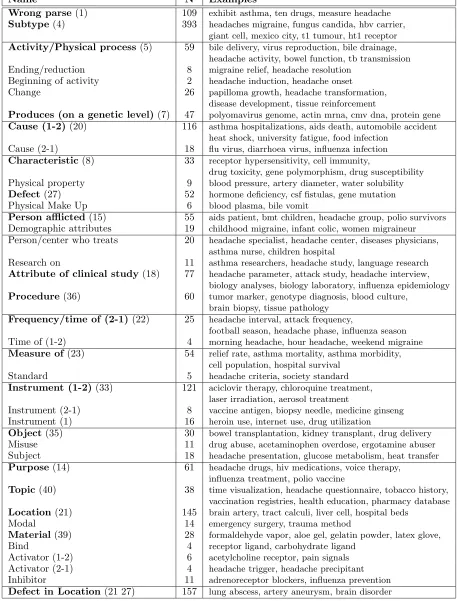
We have identified the 38 relations shown in Ta-ble 1. We tried to produce relations that correspond to the linguistic theories such as those of Levi and Warren, but in many cases these are inappropriate. Levi’s classes are too general for our purposes; for example, she collapses the “location” and “time” relationships into one single class “In” and there-fore field mouse and autumnal rain belong to the same class. Warren’s classification schema is much more detailed, and there is some overlap between the top levels of Warren’s hierarchy and our set of relations. For example, our “Cause (2-1)” for

flu viruscorresponds to her “Causer-Result” ofhay fever, and our “Person Afflicted” (migraine patient) can be thought as Warren’s “Belonging-Possessor” of gunman. Warren differentiates some classes also on the basis of the semantics of the constituents, so that, for example, the “Time” relationship is di-vided up into “Time-Animate Entity” of weekend guestsand “Time-Inanimate Entity” ofSunday pa-per. Our classification is based on the kind of re-lationships that hold between the constituent nouns rather than on the semantics of the head nouns.

For the automatic classification task, we used only the 18 relations (indicated in bold in Table 1) for which an adequate number of examples were found in the current collection. Many NCs were ambigu-ous, in that they could be described by more than one semantic relationship. In these cases, we sim-ply multi-labeled them: for example,cell growth is both “Activity” and “Change”,tumor regression is “Ending/reduction” and “Change” andbladder dys-functionis “Location” and “Defect”. Our approach handles this kind of multi-labeled classification.

Two relation types are especially problematic. Some compounds are non-compositional or lexical-ized, such as vitamin kand e2 protein; others defy classification because the nouns are subtypes of one another. This group includes migraine headache,

guinea pig, andhbv carrier. We placed all these NCs in a catch-all category. We also included a “wrong” category containing word pairs that were incorrectly labeled as NCs.2

The relations were found by iterative refinement based on looking at 2245 extracted compounds (de-scribed in the next section) and finding commonal-ities among them. Labeling was done by the au-thors of this paper and a biology student; the NCs were classified out of context. We expect to con-tinue development and refinement of these relation-ship types, based on what ends up clearly being

use-2_{The percentage of the word pairs extracted that were not}

true NCs was about 6%;some examples are: treat migraine,

ten patient,headache more. We do not know, however, how many NCs we missed. The errors occurred when the wrong label was assigned by the tagger (see Section 4).

ful “downstream” in the analysis.

The end goal is to combine these relationships in NCs with more that two constituent nouns, like in the example intranasal migraine treatment of Sec-tion 1.

4

Collection and Lexical Resources

To create a collection of noun compounds, we per-formed searches from MedLine, which contains ref-erences and abstracts from 4300 biomedical journals. We used several query terms, intended to span across different subfields. We retained only the titles and the abstracts of the retrieved documents. On these titles and abstracts we ran a part-of-speech tagger (Cutting et al., 1991) and a program that extracts only sequences of units tagged as nouns. We ex-tracted NCs with up to 6 constituents, but for this paper we consider only NCs with 2 constituents.

The Unified Medical Language System (UMLS) is a biomedical lexical resource produced and maintained by the National Library of Medicine (Humphreys et al., 1998). We use the MetaThe-saurus component to map lexical items into unique concept IDs (CUIs).3 _{The UMLS also has a}

map-ping from these CUIs into the MeSH lexical hier-archy (Lowe and Barnett, 1994); we mapped the CUIs into MeSH terms. There are about 19,000 unique main terms in MeSH, as well as additional modifiers. There are 15 main subhierarchies (trees) in MeSH, each corresponding to a major branch of medical ontology. For example, tree A cor-responds to Anatomy, tree B to Organisms, and so on. The longer the name of the MeSH term, the longer the path from the root and the more precise the description. For example migraine is C10.228.140.546.800.525, that is, C (a disease), C10 (Nervous System Diseases), C10.228 (Central Ner-vous System Diseases) and so on.

We use the MeSH hierarchy for generalization across classes of nouns; we use it instead of the other resources in the UMLS primarily because of MeSH’s hierarchical structure. For these experiments, we considered only those noun compounds for which both nouns can be mapped into MeSH terms, re-sulting in a total of 2245 NCs.

5

Method and Results

Because we have defined noun compound relation determination as a classification problem, we can make use of standard classification algorithms. In particular, we used neural networks to classify across all relations simultaneously.

3_{In some cases a word maps to more than one CUI;for the}

Name N Examples

Wrong parse(1) 109 exhibit asthma, ten drugs, measure headache

Subtype(4) 393 headaches migraine, fungus candida, hbv carrier, giant cell, mexico city, t1 tumour, ht1 receptor

Activity/Physical process(5) 59 bile delivery, virus reproduction, bile drainage, headache activity, bowel function, tb transmission

Ending/reduction 8 migraine relief, headache resolution

Beginning of activity 2 headache induction, headache onset

Change 26 papilloma growth, headache transformation,

disease development, tissue reinforcement

Produces (on a genetic level)(7) 47 polyomavirus genome, actin mrna, cmv dna, protein gene

Cause (1-2)(20) 116 asthma hospitalizations, aids death, automobile accident heat shock, university fatigue, food infection

Cause (2-1) 18 flu virus, diarrhoea virus, influenza infection

Characteristic(8) 33 receptor hypersensitivity, cell immunity,

drug toxicity, gene polymorphism, drug susceptibility

Physical property 9 blood pressure, artery diameter, water solubility

Defect(27) 52 hormone deficiency, csf fistulas, gene mutation

Physical Make Up 6 blood plasma, bile vomit

Person afflicted(15) 55 aids patient, bmt children, headache group, polio survivors

Demographic attributes 19 childhood migraine, infant colic, women migraineur

Person/center who treats 20 headache specialist, headache center, diseases physicians, asthma nurse, children hospital

Research on 11 asthma researchers, headache study, language research

Attribute of clinical study(18) 77 headache parameter, attack study, headache interview, biology analyses, biology laboratory, influenza epidemiology

Procedure(36) 60 tumor marker, genotype diagnosis, blood culture, brain biopsy, tissue pathology

Frequency/time of (2-1)(22) 25 headache interval, attack frequency,

football season, headache phase, influenza season

Time of (1-2) 4 morning headache, hour headache, weekend migraine

Measure of(23) 54 relief rate, asthma mortality, asthma morbidity, cell population, hospital survival

Standard 5 headache criteria, society standard

Instrument (1-2)(33) 121 aciclovir therapy, chloroquine treatment, laser irradiation, aerosol treatment

Instrument (2-1) 8 vaccine antigen, biopsy needle, medicine ginseng

Instrument (1) 16 heroin use, internet use, drug utilization

Object(35) 30 bowel transplantation, kidney transplant, drug delivery

Misuse 11 drug abuse, acetaminophen overdose, ergotamine abuser

Subject 18 headache presentation, glucose metabolism, heat transfer

Purpose(14) 61 headache drugs, hiv medications, voice therapy, influenza treatment, polio vaccine

Topic(40) 38 time visualization, headache questionnaire, tobacco history, vaccination registries, health education, pharmacy database

Location(21) 145 brain artery, tract calculi, liver cell, hospital beds

Modal 14 emergency surgery, trauma method

Material(39) 28 formaldehyde vapor, aloe gel, gelatin powder, latex glove,

Bind 4 receptor ligand, carbohydrate ligand

Activator (1-2) 6 acetylcholine receptor, pain signals

Activator (2-1) 4 headache trigger, headache precipitant

Inhibitor 11 adrenoreceptor blockers, influenza prevention

Defect in Location(21 27) 157 lung abscess, artery aneurysm, brain disorder

flu vaccination Model 2 D 4 G 3

Model 3 D 4 808 G 3 770 Model 4 D 4 808 54 G 3 770 Model 5 D 4 808 54 79 G 3 770 670

Model 6 D 4 808 54 79 429 G 3 770 670 310

Table 2: Different lengths of the MeSH descriptors for the different models

Model Feature Vector

2 42

3 315

4 687

5 950

6 1111

Lexical 1184

Table 3: Length of the feature vectors for different models.

We ran the experiments creating models that used different levels of the MeSH hierarchy. For example, for the NC flu vaccination, flu maps to the MeSH term D4.808.54.79.429.154.349 and vaccination to G3.770.670.310.890. Flu vaccination for Model 4 would be represented by a vector consisting of the concatenation of the two descriptors showing only the first four levels: D4.808.54.79 G3.770.670.310 (see Table 2). When a word maps to a general MeSH term (like treatment, Y11) zeros are appended to the end of the descriptor to stand in place of the missing values (so, for example, treatment in Model 3 is Y 11 0, and in Model 4 is Y 11 0 0, etc.).

The numbers in the MeSH descriptors are cate-gorical values; we represented them with indicator variables. That is, for each variable we calculated the number of possible categoriesc and then repre-sented an observation of the variable as a sequence of

c binary variables in which one binary variable was one and the remaining c−1 binary variables were zero.

We also used a representation in which the words themselves were used as categorical input variables (we call this representation “lexical”). For this col-lection of NCs there were 1184 unique nouns and therefore the feature vector for each noun had 1184 components. In Table 3 we report the length of the feature vectors for one noun for each model. The en-tire NC was described by concatenating the feature vectors for the two nouns in sequence.

The NCs represented in this fashion were used as input to a neural network. We used a feed-forward network trained with conjugate gradient descent.

Model Acc1 Acc2 Acc3

Lexical: Log Reg 0.31 0.58 0.62 Lexical: NN 0.62 0.73 0.78

2 0.52 0.65 0.72

3 0.58 0.70 0.76

4 0.60 0.70 0.76

5 0.60 0.72 0.78

6 0.61 0.71 0.76

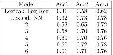
Table 4: Test accuracy for each model, where the model number corresponds to the level of the MeSH hierarchy used for classification. Lexical NN is Neural Network on Lexical and Lexical: Log Reg is Logistic Regression on NN. Acc1 refers to how often the correct relation is the top-scoring relation, Acc2 refers to how often the correct relation is one of the top two according to the neural net, and so on. Guessing would yield a result of 0.077.

The network had one hidden layer, in which a hy-perbolic tangent function was used, and an output layer representing the 18 relations. A logistic sig-moid function was used in the output layer to map the outputs into the interval (0,1).

The number of units of the output layer was the number of relations (18) and therefore fixed. The network was trained for several choices of numbers of hidden units; we chose the best-performing networks based on training set error for each of the models. We subsequently tested these networks on held-out testing data.

We compared the results with a baseline in which logistic regression was used on the lexical features. Given the indicator variable representation of these features, this logistic regression essentially forms a table of log-odds for each lexical item. We also com-pared to a method in which the lexical indicator vari-ables were used as input to a neural network. This approach is of interest to see to what extent, if any, the MeSH-based features affect performance. Note also that this lexical neural-network approach is fea-sible in this setting because the number of unique words is limited (1184) – such an approach would not scale to larger problems.

In Table 4 and in Figure 1 we report the results from these experiments. Neural network using lex-ical features only yields 62% accuracy on average across all 18 relations. A neural net trained on Model 6 using the MeSH terms to represent the nouns yields an accuracy of 61% on average across all 18 relations. Note that reasonable performance is also obtained for Model 2, which is a much more gen-eral representation. Table 4 shows that both meth-ods achieve up to 78% accuracy at including the cor-rect relation among the top three hypothesized.

2 3 4 5 6 0

0.1 0.2 0.3 0.4 0.5 0.6 0.7 0.8 0.9 1

Testing set performance on the best models for each MeSH level

Levels of the MeSH Hierarchy

Accuracy on test set

Accuracy for the largest NN output within 2 largest NN output within 3 largest NN output

Figure 1: Accuracies on the test sets for all the models. The dotted line at the bottom is the accuracy of guess-ing (the inverse of the number of classes). The dash-dot line above this is the accuracy of logistic regression on the lexical data. The solid line with asterisks is the ac-curacy of our representation, when only the maximum output value from the network is considered. The solid line with circles if the accuracy of getting the right an-swer within the two largest output values from the neural network and the last solid line with diamonds is the ac-curacy of getting the right answer within the first three outputs from the network. The three flat dashed lines are the corresponding performances of the neural net-work on lexical inputs.

the algorithm guesses yields about 5% accuracy. We see that our method is a significant improvement over the tabular logistic-regression-based approach, which yields an accuracy of only 31 percent. Addi-tionally, despite the significant reduction in raw in-formation content as compared to the lexical repre-sentation, the MeSH-based neural network performs as well as the lexical-based neural network. (And we again stress that the lexical-based neural network is not a viable option for larger domains.)

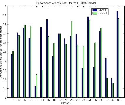
Figure 2 shows the results for each relation. MeSH-based generalization does better on some re-lations (for example 14 and 15) and Lexical on others (7, 22). It turns out that the test set for relation-ship 7 (“Produces on a genetic level”) is dominated by NCs containing the words alleles and mrnaand thatallthe NCs in the training set containing these words are assigned relation label 7. A similar situa-tion is seen for relasitua-tion 22, “Time(2-1)”. In the test set examples the second noun is either recurrence,

seasonortime. In the training set, these nouns ap-pearonlyin NCs that have been labeled as belonging to relation 22.

On the other hand, if we look at relations 14 and 15, we find a wider range of words, and in some cases

1 4 5 7 8 14 15 18 20 21 22 23 27 33 35 36 39 40 2027 0

0.1 0.2 0.3 0.4 0.5 0.6 0.7 0.8 0.9 1

Performance of each class for the LEXICAL model

Classes

Accuracies on the test set for the best model

MeSH Lexical

Figure 2:Accuracies for each class. The numbers at the bottom refer to the class numbers in Table 1. Note the very high accuracy for the “mixed” relationship 20-27 (last bar on the right).

the words in the test set are not present in the train-ing set. In relationship 14 (“Purpose”), for example,

vaccineappears 6 times in the test set (e.g.,varicella vaccine). In the training set, NCs with vaccine in it have also been classified as “Instrument” ( anti-gen vaccine, polysaccharide vaccine), as “Object” (vaccine development), as “Subtype of” (opv vac-cine) and as “Wrong” (vaccines using). Other words in the test set for 14 arevaricella which is present in the trainig set only in varicella serology labeled as “Attribute of clinical study”, drainage which is in the training set only as “Location” (gallbladder drainage and tract drainage) and “Activity” (bile drainage). Other test set words such as immunisa-tion and carcinogen do not appear in the training set at all.

In other words, it seems that the MeSHk-based categorization does better when generalization is re-quired. Additionally, this data set is “dense” in the sense that very few testing words are not present in the training data. This is of course an unrealistic situation and we wanted to test the robustness of the method in a more realistic setting. The results reported in Table 4 and in Figure 1 were obtained splitting the data into 50% training and 50% testing for each relation and we had a total of 855 training points and 805 test points. Of these, only 75 ex-amples in the testing set consisted of NCs in which both words were not present in the training set.

Model All test 1 2 3 4 Lexical: NN 0.23 0.54 0.14 0.33 0.08

2 0.44 0.62 0.25 0.53 0.38

3 0.41 0.62 0.18 0.47 0.35

4 0.42 0.58 0.26 0.39 0.38

5 0.46 0.64 0.28 0.54 0.40

6 0.44 0.64 0.25 0.50 0.39

Table 5: Test accuracy for the four sub-partitions of the test set.

and partitioned the testing set into 4 subsets as fol-lows (the numbers in parentheses are the numbers of points for each case):

• Case 1: NCs for which the first noun was not present in the training set (424)

• Case 2: NCs for which the second noun was not present in the training set (252)

• Case 3: NCs for which both nouns were present in the training set (101)

• Case 4: NCs for which both nouns were not present in the training set (810).

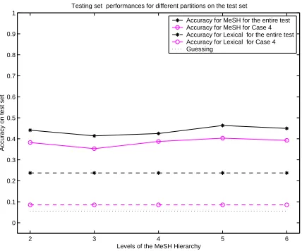
Table 5 and Figures 3 and 4 present the accuracies for these test set partitions. Figure 3 shows that the MeSH-based models are more robust than the lexical when the number of unseen words is high and when the size of training set is (very) small. In this more realistic situation, the MeSH models are able to generalize over previously unseen words. For unseen words, lexical reduces to guessing.4

Figure 4 shows the accuracy for the MeSH based-model for the the four cases of Table 5. It is interest-ing to note that the accuracy for Case 1 (first noun not present in the training set) is much higher than the accuracy for Case 2 (second noun not present in the training set). This seems to indicate that the second noun is more important for the classification that the first one.

6

Conclusions

We have presented a simple approach to corpus-based assignment of semantic relations for noun compounds. The main idea is to define a set of rela-tions that can hold between the terms and use stan-dard machine learning techniques and a lexical hi-erarchy to generalize from training instances to new examples. The initial results are quite promising.

In this task of multi-class classification (with 18 classes) we achieved an accuracy of about 60%. These results can be compared with Vanderwende

4_{Note that for unseen words, the baseline lexical-based}

logistic regression approach, which essentially builds a tabular representation of the log-odds for each class, also reduces to random guessing.

2 3 4 5 6

0 0.1 0.2 0.3 0.4 0.5 0.6 0.7 0.8 0.9 1

Testing set performances for different partitions on the test set

Levels of the MeSH Hierarchy

Accuracy on test set

Accuracy for MeSH for the entire test Accuracy for MeSH for Case 4 Accuracy for Lexical for the entire test Accuracy for Lexical for Case 4 Guessing

Figure 3: The unbroken lines represent the MeSH mod-els accuracies (for the entire test set and for case 4) and the dashed lines represent the corresponding lexical ac-curacies. The accuracies are smaller than the previous case of Table 4 because the training set is much smaller, but the point of interest is the difference in the perfor-mance of MeSH vs. lexical in this more difficult setting. Note that lexical for case 4 reduces to random guessing.

2 3 4 5 6

0 0.1 0.2 0.3 0.4 0.5 0.6 0.7 0.8 0.9 1

Testing set performances for different partitions on the test set for the MeSH−based model

Levels of the MeSH Hierarchy

Accuracy on test set

Accuracy for the entire test Case 3

Case 1 Case 2 Case 4

Figure 4: Accuracy for the MeSH based-model for the the four cases. All these curves refer to the case of get-ting exactly the right answer. Note the difference in performance between case 1 (first noun not present in the training set) and case 2 (second noun not present in training set).

(1994) who reports an accuracy of 52% with 13 classes and Lapata (2000) whose algorithm achieves about 80% accuracy for a much simpler binary clas-sification.

de-spite a somewhat errorful mapping from terms to concepts. We have also shown that representing the nouns of the compound by a very general represen-tation (Model 2) achieves a reasonable performance of aout 52% accuracy on average. This is particu-larly important in the case of larger collections with a much bigger number of unique words for which the lexical-based model is not a viable option. Our results seem to indicate that we do not lose much in terms of accuracy using the more compact MeSH representation.

We have also shown how MeSH-besed models out perform a lexical-based approach when the num-ber of training points is small and when the test set consists of words unseen in the training data. This indicates that the MeSH models can generalize successfully over unseen words. Our approach han-dles “mixed-class” relations naturally. For the mixed class Defect in Location, the algorithm achieved an accuracy around 95% for both “Defect” and “Loca-tion” simultaneously. Our results also indicate that the second noun (the head) is more important in determining the relationships than the first one.

In future we plan to train the algorithm to allow different levels for each noun in the compound. We also plan to compare the results to the tree cut algo-rithm reported in (Li and Abe, 1998), which allows different levels to be identified for different subtrees. We also plan to tackle the problem of noun com-pounds containing more than two terms.

Acknowledgments

We would like to thank Nu Lai for help with the classification of the noun compound relations. This work was supported in part by NSF award number IIS-9817353.

References

Eric Brill and Philip Resnik. 1994. A rule-based approach to prepositional phrase attachment dis-amibuation. InProceedings of COLING-94. Claire Cardie. 1997. Empirical methods in

informa-tion extracinforma-tion. AI Magazine, 18(4).

Douglass R. Cutting, Julian Kupiec, Jan O. Peder-sen, and Penelope Sibun. 1991. A practical part-of-speech tagger. In The 3rd Conference on Ap-plied Natural Language Processing, Trento, Italy. P. Downing. 1977. On the creation and use of

en-glish compound nouns. Language, (53):810–842. Christiane Fellbaum, editor. 1998. WordNet: An

Electronic Lexical Database. MIT Press.

Timothy W. Finin. 1980. The Semantic

Interpreta-tion of Compound Nominals. Ph.d. dissertaInterpreta-tion, University of Illinois, Urbana, Illinois.

Marti A. Hearst. 1990. A hybrid approach to re-stricted text interpretation. In Paul S. Jacobs, ed-itor, Text-Based Intelligent Systems: Current Re-search in Text Analysis, Information Extraction, and Retrieval, pages 38–43. GE Research & De-velopment Center, TR 90CRD198.

Donald Hindle and Mats Rooth. 1993. Structual ambiguity and lexical relations. Computational Linguistics, 19(1).

Jerry R. Hobbs, Mark Stickel, Douglas Appelt, and Paul Martin. 1993. Interpretation as abduction. Artificial Intelligence, 63(1-2).

L. Humphreys, D.A.B. Lindberg, H.M. Schoolman, and G. O. Barnett. 1998. The unified medical language system: An informatics research collab-oration. Journal of the American Medical Infor-matics Assocation, 5(1):1–13.

Maria Lapata. 2000. The automatic interpretation of nominalizations. InAAAI Proceedings.

Mark Lauer and Mark Dras. 1994. A probabilistic model of compound nouns. In Proceedings of the 7th Australian Joint Conference on AI.

Mark Lauer. 1995. Corpus statistics meet the com-pound noun. In Proceedings of the 33rd Meeting of the Association for Computational Linguistics, June.

Judith Levi. 1978. The Syntax and Semantics of Complex Nominals. Academic Press, New York. Hang Li and Naoki Abe. 1998. Generalizing case

frames using a thesaurus and the MDI principle. Computational Linguistics, 24(2):217–244. Mark Liberman and Richard Sproat. 1992. The

stress and structure of modified noun phrases in english. In I.l Sag and A. Szabolsci, editors, Lex-ical Matters. CSLI Lecture Notes No. 24, Univer-sity of Chicago Press.

Henry J. Lowe and G. Octo Barnett. 1994. Un-derstanding and using the medical subject head-ings (MeSH) vocabulary to perform literature searches. Journal of the American Medical Asso-cation (JAMA), 271(4):1103–1108.

Hwee Tou Ng and John Zelle. 1997. Corpus-based approaches to semantic interpretation in natural language processing. AI Magazine, 18(4).

James Pustejovsky, Sabine Bergler, and Peter An-ick. 1993. Lexical semantic techniques for corpus analysis. Computational Linguistics, 19(2). Philip Resnik and Marti A. Hearst. 1993. Structural

ambiguity and conceptual relations. In Proceed-ings of the ACL Workshop on Very Large Corpora, Columbus, OH.

Decem-ber. (Institute for Research in Cognitive Science report IRCS-93-42).

Philip Resnik. 1995. Disambiguating noun group-ings with respect to WordNet senses. In Third Workshop on Very Large Corpora. Association for Computational Linguistics.

Ellen Riloff. 1996. Automatically generating ex-traction patterns from untagged text. In Pro-ceedings of the Thirteenth National Conference on Artificial Intelligence and the Eighth Innovative Applications of Artificial Intelligence Conference, Menlo Park. AAAI Press / MIT Press.

Thomas Rindflesch, Lorraine Tanabe, John N. We-instein, and Lawrence Hunter. 2000. Extraction of drugs, genes and relations from the biomedical literature. Pacific Symposium on Biocomputing, 5(5).

Don R. Swanson and N. R. Smalheiser. 1994. As-sessing a gap in the biomedical literature: Mag-nesium deficiency and neurologic disease. Neuro-science Research Communications, 15:1–9. Len Talmy. 1985. Force dynamics in language and

thought. InParasession on Causatives and Agen-tivity, University of Chicago. Chicago Linguistic Society (21st Regional Meeting).

Lucy Vanderwende. 1994. Algorithm for automatic interpretation of noun sequences. In Proceedings of COLING-94, pages 782–788.

V. Vapnik. 1998. Statistical Learning Theory. Ox -ford University Press.