The Leaf Path Projection View of Parse Trees: Exploring String Kernels for HPSG Parse Selection

The Leaf Projection Path View of Parse Trees: Exploring String Kernels for

HPSG Parse Selection

Kristina Toutanova CS Dept, Stanford University

353 Serra Mall Stanford 94305, CA

USA,

[email protected]

Penka Markova EE Dept, Stanford University

350 Serra Mall Stanford 94305, CA,

USA,

[email protected]

Christopher Manning CS Dept, Stanford University

353 Serra Mall Stanford 94305, CA,

USA,

[email protected]

Abstract

We present a novel representation of parse trees as lists of paths (leaf projection paths) from leaves to the top level of the tree. This representation allows us to achieve significantly higher accuracy in the task ofHPSGparse selection than standard models, and makes the application of string kernels natural. We define tree kernels via string kernels on projec-tion paths and explore their performance in the con-text of parse disambiguation. We apply SVM rank-ing models and achieve an exact sentence accuracy of 85.40% on the Redwoods corpus.

1 Introduction

In this work we are concerned with building sta-tistical models for parse disambiguation – choos-ing a correct analysis out of the possible analyses for a sentence. Many machine learning algorithms for classification and ranking require data to be rep-resented as real-valued vectors of fixed dimension-ality. Natural language parse trees are not readily representable in this form, and the choice of repre-sentation is extremely important for the success of machine learning algorithms.

For a large class of machine learning algorithms, such an explicit representation is not necessary, and it suffices to devise a kernel function which measures the similarity between inputs

and

. In addition to achieving efficient computation in high dimensional representation spaces, the use of ker-nels allows for an alternative view on the mod-elling problem as defining a similarity between in-puts rather than a set of relevant features.

In previous work on discriminative natural lan-guage parsing, one approach has been to define fea-tures centered around lexicalized local rules in the trees (Collins, 2000; Shen and Joshi, 2003), simi-lar to the features of the best performing lexicalized generative parsing models (Charniak, 2000; Collins, 1997). Additionally non-local features have been defined measuring e.g. parallelism and complexity of phrases in discriminative log-linear parse ranking

models (Riezler et al., 2000).

Another approach has been to define tree kernels: for example, in (Collins and Duffy, 2001), the all-subtrees representation of parse trees (Bod, 1998) is effectively utilized by the application of a fast dynamic programming algorithm for computing the number of common subtrees of two trees. Another tree kernel, more broadly applicable to Hierarchi-cal Directed Graphs, was proposed in (Suzuki et al., 2003). Many other interesting kernels have been de-vised for sequences and trees, with application to se-quence classification and parsing. A good overview of kernels for structured data can be found in (Gaert-ner et al., 2002).

Here we propose a new representation of parse trees which (i) allows the localization of broader useful context, (ii) paves the way for exploring ker-nels, and (iii) achieves superior disambiguation ac-curacy compared to models that use tree representa-tions centered around context-free rules.

Compared to the usual notion of discriminative models (placing classes on rich observed data) dis-criminative PCFG parsing with plain context free rule features may look naive, since most of the fea-tures (in a particular tree) make no reference to ob-served input at all. The standard way to address this problem is through lexicalization, which puts an el-ement of the input on each tree node, so all features do refer to the input. This paper explores an alterna-tive way of achieving this that gives a broader view of tree contexts, extends naturally to exploring ker-nels, and performs better.

We represent parse trees as lists of paths (leaf

pro-jection paths) from words to the top level of the tree,

IMPERverb

HCOMPverb

HCOMPverb

LET V1

let

US

us

HCOMPverb

PLAN ON V2

plan

HCOMPprep*

ON

on

THAT DEIX

that

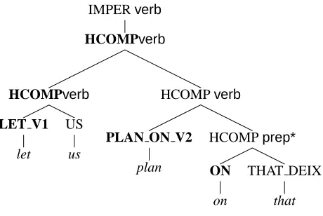
Figure 1: Derivation tree for the sentence Let us

plan on that.

paths (strings) allows us to explore string kernels on these paths and combine them into tree kernels.

We apply these ideas in the context of parse disambiguation for sentence analyses produced by a Head-driven Phrase Structure Grammar (HPSG), the grammar formalism underlying the Redwoods corpus (Oepen et al., 2002). HPSG is a modern constraint-based lexicalist (or “unification”) gram-mar formalism.1 We build discriminative mod-els using Support Vector Machines for ranking (Joachims, 1999). We compare our proposed rep-resentation to previous approaches and show that it leads to substantial improvements in accuracy.

2 The Leaf Projection Paths View of Parse Trees

2.1 Representing HPSG Signs

In HPSG, sentence analyses are given in the form of HPSG signs, which are large feature structures

containing information about syntactic and seman-tic properties of the phrases.

As in some of the previous work on the Red-woods corpus (Toutanova et al., 2002; Toutanova and Manning, 2002), we use the derivation trees as the main representation for disambiguation. Deriva-tion trees record the combining rule schemas of the HPSG grammar which were used to license the sign by combining initial lexical types. The derivation tree is also the fundamental data stored in the Redwoods treebank, since the full sign can be reconstructed from it by reference to the gram-mar. The internal nodes represent, for example, head-complement, head-specifier, and head-adjunct schemas, which were used to license larger signs out of component parts. A derivation tree for the

1

For an introduction toHPSG, see (Pollard and Sag, 1994).

IMPERverb

HCOMPverb

HCOMPverb

LET V1

let (v sorb)

IMPERverb

HCOMPverb

HCOMPverb

PLAN ON V2

plan (v e p itrs)

IMPERverb

HCOMPverb

HCOMPverb

HCOMPprep*

ON

on (p reg)

Figure 2: Paths to top for three leaves. The nodes in bold are head nodes for the leaf word and the rest are non-head nodes.

sentence Let us plan on that is shown in Figure 1. 2 Additionally, we annotate the nodes of the deriva-tion trees with informaderiva-tion extracted from theHPSG

sign. The annotation of nodes is performed by ex-tracting values of feature paths from the feature structure or by propagating information from chil-dren or parents of a node. In theory with enough annotation at the nodes of the derivation trees, we can recover the wholeHPSGsigns.

Here we describe three node annotations that proved very useful for disambiguation. One is annotation with the values of the feature path synsem.local.cat.head– its values are basic parts of speech such as noun, verb, prep, adj, adv. An-other is phrase structure category information asso-ciated with the nodes, which summarizes the values of several feature paths and is available in the Red-woods corpus as Phrase-Structure trees. The third is annotation with lexical type (le-type), which is the type of the head word at a node. The preterminals in Figure 1 are lexical item identifiers — identifiers of the lexical entries used to construct the parse. The

le-types are about types in theHPSGtype

hier-archy and are the direct super-types of the lexical item identifiers. The le-types are not shown in this figure, but can be seen at the leaves in Figure 2. For example, the lexical type of LET V1 in the figure is

v sorb. In Figure 1, the only annotation performed

is with the values ofsynsem.local.cat.head.

2.2 The Leaf Projection Paths View

The projection path of a leaf is the sequence of nodes from the leaf to the root of the tree. In Figure 2, the leaf projection paths for three of the words are shown.

We can see that a node in the derivation tree

par-2

ticipates in the projection paths of all words domi-nated by that node. The original local rule config-urations — a node and its children, do not occur jointly in the projection paths; thus, if special anno-tation is not performed to recover it, this informa-tion is lost.

As seen in Figure 2, and as is always true for a grammar that produces non-crossing lexical depen-dencies, there is an initial segment of the projec-tion path for which the leaf word is a syntactic head (called head path from here on), and a final segment for which the word is not a syntactic head (called

non-head path from here on). In HPSG non-local

dependencies are represented in the final semantic representation, but can not be obtained via syntactic head annotation.

If, in a traditional parsing model that estimates the likelihood of a local rule expansion given a node (such as e.g (Collins, 1997)), the tree nodes are an-notated with the word of the lexical head, some in-formation present in the word projection paths can be recovered. However, this is only the information in the head path part of the projection path. In fur-ther experiments we show that the non-head part of the projection path is very helpful for disambigua-tion.

Using this representation of derivation trees, we can apply string kernels to the leaf projection paths and combine those to obtain kernels on trees. In the rest of this paper we explore the application of string kernels to this task, comparing the performance of the new models to models using more standard rule features.

3 Tree and String Kernels

3.1 Kernels and SVM ranking

From a machine learning point of view, the parse se-lection problem can be formulated as follows: given

training examples (

, where each is a natural language sentence, is

the number of such sentences,

, is

a parse tree for , is the number of parses for a

given sentence,

is a feature representation

for the parse tree

, and we are given the training

information which of all

is the correct parse –

learn how to correctly identify the correct parse of an unseen test sentence.

One approach for solving this problem is via representing it as an SVM (Vapnik, 1998) ranking problem, where (without loss of generality)

is

assumed to be the correct parse for . The goal is

to learn a parameter vector

, such that the score of

(

) is higher than the scores of all other

parses for the sentence. Thus we optimize for:

"!$#

% &

('()+* ,

-/."0 213

& 4

657

98

5

,

-/."0 21

,

8

The ,

are slack variables used to handle the

non-separable case. The same formulation has been used in (Collins, 2001) and (Shen and Joshi, 2003). This problem can be solved by solving the dual, and thus we would only need inner products of the feature vectors. This allows for using the kernel trick, where we replace the inner product in the representation space by inner product in some fea-ture space, usually different from the representation space. The advantage of using a kernel is associ-ated with the computational effectiveness of com-puting it (it may not require performing the expen-sive transformation

explicitly).

We learn SVM ranking models using a tree kernel defined via string kernels on projection paths.

3.2 Kernels on Trees Based on Kernels on Projection Paths

So far we have defined a representation of parse trees as lists of strings corresponding to projection paths of words. Now we formalize this representa-tion and show how string kernels on projecrepresenta-tion paths extend to tree kernels.

We introduce the notion of a keyed string — a string that has a key, which is some letter from the alphabet : of the string. We can denote a keyed

string by a pair <;

, where ;>=

: is the key,

and

is the string. In our application, a key would be a word

, and the string would be the sequence of derivation tree nodes on the head or non-head part of the projection path of the word

. Addi-tionally, for reducing sparsity, for each keyed string

, we also include a keyed string <?A@B

, where?A@B

is the le-type of the word

. Thus each projection path occurs twice in the list representa-tion of the tree – once headed by the word, and once by its le-type. In our application, the strings

are sequences of annotated derivation tree nodes, e.g.

=“LET V1:verb HCOMP:verb HCOMP:verb IM-PER:verb” for the head projection path of let in Fig-ure 2. The non-head projection path of let is empty. For a given kernel on strings, we de-fine its extension to keyed strings as follows:

<; AC

, if ;

C

, and

<; AC

, otherwise. We use this

Given a tree 3 and a tree AC AC

, and a kernel on keyed strings, we define a kernel on the trees as follows: * * <; AC

This can be viewed as a convolution (Haussler, 1999) and therefore is a valid kernel (positive definite symmetric), if is a valid kernel.

3.3 String Kernels

We experimented with some of the string kernels proposed in (Lodhi et al., 2000; Leslie and Kuang, 2003), which have been shown to perform very well for indicating string similarity in other domains. In particular we applied the N-gram kernel, Subse-quence kernel, and Wildcard kernel. We refer the reader to (Lodhi et al., 2000; Leslie and Kuang, 2003) for detailed formal definition of these ker-nels, and restrict ourselves to an intuitive descrip-tion here. In addidescrip-tion, we devised a new kernel, called Repetition kernel, which we describe in de-tail.

The kernels used here can be defined as the in-ner product of the feature vectors of the two strings

( , )= x (

), with feature map from the space of all finite sequences from a string alpha-bet : to a vector space indexed by a set of

sub-sequences from : . As a simple example, the

-gram string kernel maps each string =

: to a

vector with dimensionality : and each element in

the vector indicates the number of times the corre-sponding symbol from: occurs in

. For example,

<; C ; ;

.

The Repetition kernel is similar to the 1-gram ker-nel. It improves on the -gram kernel by better

han-dling cases with repeated occurrences of the same symbol. Intuitively, in the context of our applica-tion, this kernel captures the tendency of words to take (or not take) repeated modifiers of the same kind. For example, it may be likely that a ceratin verb take one PP-modifier, but less likely for it to take two or more.

More specifically, the Repetition kernel is defined such that its vector space consists of all sequences from : composed of the same symbol. The

fea-ture map obtains matching of substrings of the in-put string to features, allowing the occurrence of gaps. There are two discount parameters and

. serves to discount features for the occurrence of gaps, and

discounts longer symbol sequences. Formally, for an input string

, the value of the feature vector for the feature index sequence !

, !"3$# , is defined as follows: Let be

the left-most minimal contiguous substring of

that contains ! , 7

&%, where for indices

' ? , )( ; *3

+ . Then -,/. .0 0 21 3 ( )= % ' ' .

For our previous example, if

,

<; C4 ; ;

,

5

<; C4 ; ;

% , and 5

<; C4 ; ;

%

.

The weighted Wildcard kernel performs match-ing by permittmatch-ing a restricted number of matches to a wildcard character. A

#

wildcard kernel has as feature indices # -grams with up to wildcard

characters. Any character matches a wildcard. For example the 3-gram

; ; C

will match the feature in-dex ;76 C

in a (3,1) wildcard kernel. The weighting is based on the number of wildcard characters used – the weight is multiplied by a discount for each wildcard.

The Subsequence kernel was defined in (Lodhi et al., 2000). We used a variation where the ker-nel is defined by two integers

#

8

and two dis-count factors and

for gaps and characters. A subseq(k,g)kernel has as features all9 -grams with

9:;# . The

8

is a restriction on the maximal span of the9 -gram in the original string – e.g. if#

%

and

8

=< , the two letters of a

%

-gram can be at most8 5

#+

%

letters apart in the original string. The weight of a feature is multiplied by 6 for each

gap, and by

for each non-gap. For the exam-ple above, if

> # % 8 > ,

<; C ; ;

@? @?

3

< . The feature

in-dex

; ;

matches only once in the string with a span at most – for the sequence

; ;

with gap.

The details of the algorithms for computing the kernels can be found in the fore-mentioned papers (Lodhi et al., 2000; Leslie and Kuang, 2003). To summarize, the kernels can be implemented effi-ciently using tries.

4 Experiments

In this section we describe our experimental results using different string kernels and different feature annotation of parse trees. We learn Support Vector Machine (SVM) ranking models using the software packageACBED

%

F5G

0

(Joachims, 1999). We also nor-malized the kernels:

IH J KL 0 ( 0 *M N KL 0 ( 0 (OM N KL 0 * 0 *M .

For all tree kernels implemented here, we first ex-tract all features, generating an explicit map to the space of the kernel, and learn SVM ranking models using APBQD

%F5G

0

the problem in its primal form. We were not aware of the existence of any fast software packages that could solve SVM ranking problems in the dual for-mulation. It is possible to convert the ranking prob-lem into a classification probprob-lem using pairs of trees as shown in (Shen and Joshi, 2003). We have taken this approach in more recent work using string ker-nels requiring very expensive feature maps.

We performed experiments using the version of the Redwoods corpus which was also used in the work of (Toutanova et al., 2002; Osborne and Bald-bridge, 2004) and others. There are

anno-tated sentences in total, %

of which are ambigu-ous. The average sentence length of the ambiguous sentences is

words and the average number of

parses per sentence is

. We discarded the

un-ambiguous sentences from the training and test sets. All models were trained and tested using 10-fold cross-validation. Accuracy results are reported as percentage of sentences where the correct analysis was ranked first by the model.

The structure of the experiments section is as fol-lows. First we describe the results from a controlled experiment using a limited number of features, and aimed at comparing models using local rule features to models using leaf projection paths in Section 4.1. Next we describe models using more sophisticated string kernels on projection paths in Section 4.2.

4.1 The Leaf Projection Paths View versus the Context-Free Rule View

In order to evaluate the gains from the new repre-sentation, we describe the features of three similar models, one using the leaf projection paths, and two using derivation tree rules. Additionally, we train a model using only the features from the head-path parts of the projection paths to illustrate the gain of using the non-head path. As we will show, a model using only the head-paths has almost the same fea-tures as a rule-based tree model.

All models here use derivation tree nodes anno-tated with only the rule schema name as in Figure 1 and the synsem.local.cat.headvalue. We will define these models by their feature map from trees to vectors. It will be convenient to define the feature maps for all models by defining the set of features through templates. The value

3

for a feature!

and tree

, will be the number of times! occurs in

the tree. It is easy to show that the kernels on trees we introduce in Section 3.2, can be defined via a feature map that is the sum of the feature maps of the string kernels on projection paths.

As a concrete example, for each model we show all features that contain the node [HCOMP:verb]

from Figure 1, which covers the phrase plan on that.

Bi-gram Model on Projection Paths (2PP)

The features of this model use a projection path representation, where the keys are not the words, but the le-types of the words. The features of this model are defined by the following template : <?A@

@ 9

@

9 @

@ ;

.

@;

is a binary variable showing whether this feature matches a head or a non-head path, ?A@

@

is the le-type of the path leaf, and9

@

9 @

is a

bi-gram from the path.

The node[HCOMP:verb]is part of the head-path for plan, and part of the non-head path for on and

that. The le-types of the words let, plan, on, and that

are, with abbreviations, v sorb, v e p, p reg, and

n deic pro sg respectively. In the following

exam-ples, the node labels are abbreviated as well;

is a special symbol for end of path and A is a

special symbol for start of path. Therefore the fea-tures that contain the node will be:

(v_e_p,[PLAN_ON:verb],[HCOMP:verb],1) (v_e_p,[HCOMP:verb],EOP,1)

(p_reg,SOP,[HCOMP:verb],0)

(p_reg,[HCOMP:verb],[HCOMP:verb],0)

(n_deic_pro_sg,[HCOMP:prep*],[HCOMP:verb],0) (n_deic_pro_sg,[HCOMP:verb],[HCOMP:verb],0)

Bi-gram Model on only Head Projection Paths (2HeadPP)

This model has a subset of the features of Model 2PP— only those obtained by the head path parts of the projection paths. For our example, it contains the subset of features of 2PP that have last bit ,

which will be only the following:

(v_e_p,[PLAN_ON:verb],[HCOMP:verb],1) (v_e_p,[HCOMP:verb],EOP,1)

Rule Tree Model I (Rule I)

The features of this model are defined by the two templates: <?A@

@ 9

@

?

?

and <?A@

@ 9

@

?)

?)

. The last value in

the tuples is an indication of whether the tuple con-tains the le-type of the head or the non-head child as its first element. The features containing the node

[HCOMP:verb] are ones from the expansion at that node and also from the expansion of its parent:

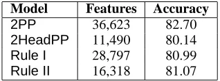
Model Features Accuracy

2PP 36,623 82.70

2HeadPP 11,490 80.14 Rule I 28,797 80.99 Rule II 16,318 81.07

Table 1: Accuracy of models using the leaf projec-tion path and rule representaprojec-tions.

Rule Tree Model II (Rule II)

This model splits the features of model Rule I in two parts, to mimic the features of the projection path models. It has features from the following tem-plates: <?<@

@ @; 9

@ @ ;

)

?)

and <?A@

@ 9

@; 9

@ 9&9

@;

)

? .

The features containing the [HCOMP:verb] node are:

(v_e_p,[HCOMP:verb],[PLAN_ON:verb],1) (p_reg,[HCOMP:verb],[HCOMP:prep*],0) (v_sorb,[HCOMP:verb],[HCOMP:verb],1) (v_e_p,[HCOMP:verb],[HCOMP:verb],0)

This model has less features than model Rule I, because it splits each rule into its head and non-head parts and does not have the two parts jointly. We can note that this model has all the features of 2HeadPP, except the ones involving start and end of path, due to the first template. The second tem-plate leads to features that are not even in2PP be-cause they connect the head and non-head paths of a word, which are represented as separate strings in 2PP.

Overall, we can see that modelsRule IandRule II have the information used by 2HeadPP (and some more information), but do not have the in-formation from the non-head parts of the paths in Model2PP. Table 1 shows the average parse rank-ing accuracy obtained by the four models as well as the number of features used by each model. Model Rule Idid not do better than modelRule II, which shows that joint representation of rule features was not very important. The large improvement of2PP over 2HeadPP (13% error reduction) shows the usefulness of the non-head projection paths. The er-ror reduction of2PPoverRule Iis also large – 9% error reduction. Further improvements over mod-els using rule features were possible by considering more sophisticated string kernels and word keyed projection paths, as will be shown in the following sections.

4.2 Experimental Results using String Kernels on Projection Paths

In the present experiments, we have limited the derivation tree node annotation to the features listed in Table 2. Many other features from theHPSGsigns

No. Name Example

0 Node Label HCOMP

1 synsem.local.cat.head verb 2 Label from Phrase Struct Tree S 3 Le Type of Lexical Head v sorb le 4 Lexical Head Word let

Table 2: Annotated features of derivation tree nodes. The examples are from one node in the head path of the word let in Figure 1.

are potentially helpful for disambiguation, and in-corporating more useful features is a next step for this work. However, given the size of the corpus, a single model can not usefully profit from a large number of features. Previous work (Osborne and Baldbridge, 2004; Toutanova and Manning, 2002; Toutanova et al., 2002) has explored combining multiple classifiers using different features. We re-port results from such an experiment as well.

Using Node Label and Head Category Annotations

The simplest derivation tree node representation that we consider consists of features and

-schema name and category of the lexical head. All experiments in this subsection section were per-formed using this derivation tree annotation. We briefly mention results from the best string-kernels when using other node annotations, as well as a combination of models using different features in the following subsection.

To evaluate the usefulness of our Repetition Ker-nel, defined in Section 3.3, we performed several simple experiments. We compared it to a -gram

kernel, and to a%

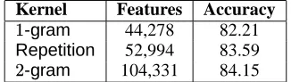
-gram kernel. The results – num-ber of features per model, and accuracy, are shown in Table 3. The models shown in this table include both features from projection paths keyed by words and projection paths keyed by le-types. The results show that the Repetition kernel achieves a notice-able improvement over a -gram model (

error

reduction), with the addition of only a small number of features. For most of the words, repeated sym-bols will not occur in their paths, and the Repetition kernel will behave like a -gram for the majority of

cases. The additional information it captures about repeated symbols gives a sizable improvement. The bi-gram kernel performs better but at the cost of the addition of many features. It is likely that for large alphabets and small training sets, the Repetition ker-nel may outperform the bi-gram kerker-nel.

Rep-Kernel Features Accuracy

-gram 44,278 82.21 Repetition 52,994 83.59

-gram 104,331 84.15

Table 3: Comparison of the Repetition kernel to

-gram and%

-gram.

etition kernel. We found that, because lexical in-formation is sparse, going beyond %

-grams for lex-ically headed paths was not useful. The projection paths keyed by le-types are much less sparse, but still capture important sequence information about the syntactic frames of words of particular lexical types.

To study the usefulness of different string kernels on projection paths, we first tested models where only le-type keyed paths were represented, and then tested the performance of the better models when word keyed paths were added (with a fixed string kernel that interpolates a bi-gram and a Repetition kernel).

Table 4 shows the accuracy achieved by several string kernels as well as the number of features (in thousands) they use. As can be seen from the ta-ble, the models are very sensitive to the discount factors used. Many of the kernels that use some combination of 1-grams and possibly discontinu-ous bi-grams performed at approximately the same accuracy level. Such are the wildcard(2,1, ) and subseq(2,8

, ,

) kernels. Kernels that use

-grams have many more parameters, and even though they can be marginally better when using le-types only, their advantage when adding word keyed paths disappears. A limited amount of discontinuity in the Subsequence kernels was useful. Overall Sub-sequence kernels were slightly better than Wild-card kernels. The major difference between the two kinds of kernels as we have used them here is that the Subsequence kernel unifies features that have gaps in different places, and the Wildcard kernel does not. For example,;@6 C 6 ; C ; C 6

are different features for Wildcard, but they are the same feature

; C

for Subsequence – only the weighting of the fea-ture depends on the position of the wildcard.

When projection paths keyed by words are added, the accuracy increases significantly. sub-seq(2,3,.5,2) achieved an accuracy of <

,

which is much higher than the best previously pub-lished accuracy from a single model on this corpus (

%

for a model that incorporates more sources

of information from the HPSG signs (Toutanova et

al., 2002)). The error reduction compared to that model is

. It is also higher than the best

re-sult from voting classifiers ( < %

(Osborne and

Model Features Accuracy

le w & le le w & le

1gram 13K - 81.43

-2gram 37K 141K 82.70 84.11

wildcard (2,1,.7) 62K 167K 83.17 83.86 wildcard (2,1,.25) 62K 167K 82.97 -wildcard (3,1,.5) 187K 291K 83.21 83.59 wildcard (3,2,.5) 220K 82.90 -subseq (2,3,.5,2) 81K 185K 83.22 84.96

subseq (2,3,.25,2) 81K 185K 83.48 84.75 subseq (2,3,.25,1) 81K 185K 82.89 -subseq (2,4,.5,2) 102K 206K 83.29 84.40 subseq (3,3,.5,2) 154K 259K 83.17 83.85 subseq (3,4,.25,2) 290K - 83.06 -subseq (3,5,.25,2) 416K - 83.06

-combination model 85.40

Table 4: Accuracy of models using projection paths keyed by le-type or both word and le-type. Numbers

of features are shown in thousands.

Baldbridge, 2004)).

Other Features and Model Combination

Finally, we trained several models using different derivation tree annotations and built a model that combined the scores from these models together with the best model subseq(2,3,.5,2) from Table 4. The combined model achieved our best accuracy of

< . The models combined were:

Model I A model that uses the Node Label and

le-type of non-head daughter for head projection paths, and Node Label and sysnem.local.cat.head for non-head projection paths. The model used the sub-seq(2,3,.5,2)kernel for le-type keyed paths and bi-gram + Repetition for word keyed paths as above. Number of features of this model: 237K Accuracy:

<

< .

Model II A model that uses, for head paths,

Node Label of node and Node Label and sys-nem.local.cat.headof non-head daughter, and for non-head paths PS category of node. The model uses the same kernels asModel I. Number of fea-tures: 311K. Accuracy:

%

.

Model III This model uses PS label and sys-nem.local.cat.head for head paths, and only PS label for non-head paths. The kernels are the same as Model I. Number of features: 165K Accuracy:

.

Model IV This is a standard model based on

rule features for local trees, with %

levels of grand-parent annotation and back-off. The annotation used at nodes was with Node Label and sys-nem.local.cat.head. Number of features: 78K Ac-curacy:

5 Conclusions

We proposed a new representation of parse trees that allows us to connect more tightly tree structures to the words of the sentence. Additionally this repre-sentation allows for the natural extension of string kernels to kernels on trees. The major source of ac-curacy improvement for our models was this rep-resentation, as even with bi-gram features, the per-formance was higher than previously achieved. We were able to improve on these results by using more sophisticated Subsequence kernels and by our Rep-etition kernel which captures some salient proper-ties of word projection paths.

In future work, we aim to explore the definition of new string kernels that are more suitable for this particular application and apply these ideas to Penn Treebank parse trees. We also plan to explore anno-tation with more features fromHPSGsigns.

Acknowledgements

We would like to thank the anonymous review-ers for helpful comments. This work was car-ried out under the Edinburgh-Stanford Link pro-gramme, funded by Scottish Enterprise, ROSIE project R36763.

References

Rens Bod. 1998. Beyond Grammar: An Experience

Based Theory of Language. CSLI Publications.

Eugene Charniak. 2000. A maximum entropy in-spired parser. In Proceedings of NAACL, pages 132 – 139.

Michael Collins and Nigel Duffy. 2001. Convolu-tion kernels for natural language. In Proceedings

of NIPS.

Michael Collins. 1997. Three generative, lexi-calised models for statistical parsing. In

Proceed-ings of the ACL, pages 16 – 23.

Michael Collins. 2000. Discriminative reranking for natural language parsing. In Proceedings of

ICML, pages 175–182.

Michael Collins. 2001. Parameter estimation for statistical parsing models: Theory and practice of distribution-free methods. In IWPT. Paper writ-ten to accompany invited talk at IWPT 2001. Thomas Gaertner, John W. Lloyd, and Peter A.

Flach. 2002. Kernels for structured data. In

ILP02, pages 66–83.

David Haussler. 1999. Convolution kernels on dis-crete structures. In UC Santa Cruz Technical

Re-port UCS-CRL-99-10.

Thorsten Joachims. 1999. Making large-scale SVM learning practical. In B. Scholkopf,

C. Burges, and A. Smola, editors, Advances in

Kernel Methods - Support Vector Learning.

Christina Leslie and Rui Kuang. 2003. Fast ker-nels for inexact string matching. In COLT 2003, pages 114–128.

Huma Lodhi, John Shawe-Taylor, Nello Cristianini, and Christopher J. C. H. Watkins. 2000. Text classification using string kernels. In

Proceed-ings of NIPS, pages 563–569.

Stephan Oepen, Kristina Toutanova, Stuart Shieber, Chris Manning, and Dan Flickinger. 2002. The LinGo Redwoods treebank: Motivation and pre-liminary apllications. In Proceedings of COLING

19, pages 1253—1257.

Miles Osborne and Jason Baldbridge. 2004. Ensemble-based active learning for parse selec-tion. In Proceedings of HLT-NAACL.

Carl Pollard and Ivan A. Sag. 1994. Head-Driven Phrase Structure Grammar. University of

Chicago Press.

Stefan Riezler, Detlef Prescher, Jonas Kuhn, and Mark Johnson. 2000. Lexicalized stochastic modeling of constraint-based grammars using log-linear measures and EM training. In

Pro-ceedings of the ACL, pages 480—487.

Libin Shen and Aravind K. Joshi. 2003. An SVM-based voting algorithm with application to parse reranking. In Proceedings of CoNLL, pages 9– 16.

Jun Suzuki, Tsutomu Hirao, Yutaka Sasaki, and Eisaku Maeda. 2003. Hierarchical directed acyclic graph kernel: Methods for structured nat-ural language data. In Proceedings of the ACL, pages 32 – 39.

Kristina Toutanova and Christopher D. Manning. 2002. Feature selection for a rich HPSG gram-mar using decision trees. In Proceedings of

CoNLL.

Kristina Toutanova, Christopher D. Manning, Stu-art Shieber, Dan Flickinger, and Stephan Oepen. 2002. Parse disambiguation for a rich HPSG grammar. In Proceedings of Treebanks and

Lin-guistic Theories, pages 253–263.

Vladimir Vapnik. 1998. Statistical Learning