Interactive Feature Space Construction using Semantic Information
Dan Roth and Kevin Small
Department of Computer Science University of Illinois at Urbana-Champaign
Urbana, IL 61801
{danr,ksmall}@illinois.edu
Abstract
Specifying an appropriate feature space is an important aspect of achieving good perfor-mance when designing systems based upon learned classifiers. Effectively incorporat-ing information regardincorporat-ing semantically related words into the feature space is known to pro-duce robust, accurate classifiers and is one ap-parent motivation for efforts to automatically generate such resources. However, naive in-corporation of this semantic information may result in poor performance due to increased ambiguity. To overcome this limitation, we introduce the interactive feature space con-struction protocol, where the learner identi-fies inadequate regions of the feature space and in coordination with a domain expert adds descriptiveness through existing semantic re-sources. We demonstrate effectiveness on an entity and relation extraction system includ-ing both performance improvements and ro-bustness to reductions in annotated data.
1 Introduction
An important natural language processing (NLP) task is the design of learning systems which per-form well over a wide range of domains with limited training data. While the NLP community has a long tradition of incorporating linguistic information into statistical systems, machine learning approaches to these problems often emphasize learning sophisti-cated models over simple, mostly lexical, features. This trend is not surprising as a primary motivation for machine learning solutions is to reduce the man-ual effort required to achieve state of the art
perfor-mance. However, one notable advantage of discrimi-native classifiers is the capacity to encode arbitrarily complex features, which partially accounts for their popularity. While this flexibility is powerful, it often overwhelms the system designer causing them to re-sort to simple features. This work presents a method to partially automate feature engineering through an interactive learning protocol.
While it is widely accepted that classifier perfor-mance is predicated on feature engineering, design-ing good features requires significant effort. One un-derutilized resource for descriptive features are ex-istingsemantically related word lists(SRWLs), gen-erated both manually (Fellbaum, 1998) and automat-ically (Pantel and Lin, 2002). Consider the follow-ing named entity recognition (NER) example:
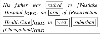
His father was rushed to [Westlake Hospital]ORG, an arm of [Resurrection Health Care]ORG, in west suburban [Chicagoland]LOC.
For such tasks, it is helpful to know that west is a member of the SRWL [Compass Direction] and other such designations. If extracting features using this information, we would require observing only a subset of the SRWL in the data to learn the cor-responding parameter. This statement suggests that one method for learning robust classifiers is to in-corporate semantic information through features ex-tracted from the more descriptive representation:
His father was rushed to Westlake [Health Care Institution], an [Subsidiary] of Resur-rection Health Care, [Locative Preposition] [Compass Direction] suburban Chicagoland.
Deriving discriminative features from this rep-resentation often results in more informative fea-tures and a correspondingly simpler classification task. Although effective approaches along this vein have been shown to induce more accurate classi-fiers (Boggess et al., 1991; Miller et al., 2004; Li and Roth, 2005), naive approaches may instead result in higher sample complexity due to increased ambi-guity introduced through these semantic resources. Features based upon SRWLs must therefore balance the tradeoff between descriptiveness and noise.
This paper introduces the interactive feature space construction (IFSC) protocol, which facil-itates coordination between a domain expert and learning algorithm to interactively define the feature space during training. This paper describes the par-ticular instance of the IFSC protocol where seman-tic information is introduced through abstraction of lexical terms in the feature space with their SRWL labels. Specifically, there are two notable contri-butions of this work: (1) an interactive method for the expert to directly encode semantic knowledge into the feature space with minimal effort and (2) a querying function which uses both the current state of the learner and properties of the available SRWLs to select informative instances for presentation to the expert. We demonstrate the effectiveness of this protocol on an entity and relation extraction task in terms of performance and labeled data requirements.
2 Preliminaries
Following standard notation, let x ∈ X represent members of an input domain and y ∈ Y represent members of an output domain where a learning al-gorithm uses a training sample S = {(xi, yi)}mi=1
to induce a prediction function h : X → Y. We
are specifically interested in discriminative classi-fiers which use a feature vector generating procedure
Φ(x) → x, taking an input domain memberx and
generating a feature vectorx. We further assume the output assignment ofhis based upon a scoring func-tionf : Φ(X)× Y →Rsuch that the prediction is stated asyˆ=h(x) = argmaxy0∈Yf(x, y0).
The feature vector generating procedure is com-posed of a vector of feature generation functions (FGFs),Φ(x) =hΦ1(x),Φ2(x), . . . ,Φn(x)i, where
each feature generation function, Φi(x) → {0,1},
takes the input x and returns the appropriate
fea-ture vector value. Consider the text “in west sub-urban Chicagoland” where we wish to predict the entity classification forChicagoland. In this case, example active FGFs include Φtext=Chicagoland,
ΦisCapitalized, andΦtext(−2)=westwhile FGFs such
asΦtext=and would remain inactive. Since we are
constructing sparse feature vectors, we use the infi-nite attribute model(Blum, 1992).
Semantically related word list (SRWL) feature abstraction begins with a set of variable sized word lists {W} such that each member lexical element (i.e. word, phrase) has at least one sense that is semantically related to the concept represented by W (e.g. Wcompass direction = north, east, . . . , southwest). For the purpose of feature extraction, whenever the sense of a lexical el-ement associated with a particularW appears in the corpus, it is replaced by the name of the correspond-ing SRWL. This is equivalent to defincorrespond-ing a FGF for the specifiedW which is a disjunction of the func-tionally related FGFs over the member lexical ele-ments (e.g. Φtext∈Wcompass direction = Φtext=north∨ Φtext=east∨. . .∨Φtext=southwest).
3 Interactive Feature Space Construction
The machine learning community has become in-creasingly interested in protocols which allow inter-action with a domain expert during training, such as the active learning protocol (Cohn et al., 1994). In active learning, the learning algorithm reduces the labeling effort by using a querying function to in-crementally select unlabeled examples from a data source for annotation during learning. By care-fully selecting examples for annotation, active learn-ing maximizes the quality of inductive information while minimizing label acquisition cost.
Learning algorithms generally assume that the feature space and model are specified before learn-ing begins and remain static throughout learnlearn-ing, where training data is exclusively used for parameter estimation. Conversely, theinteractive feature space construction(IFSC) protocol relaxes this static fea-ture space assumption by using information about the current state of the learner, properties of knowl-edge resources (e.g. SRWLs, gazetteers, unlabeled data, etc.), and access to the domain expert during training to interactively improve the feature space. Whereas active learning focuses on the labeling ef-fort, IFSC reduces sample complexity and improves performance by modifying the underlying represen-tation to simplify the overall learning task.
The IFSC protocol for SRWL abstraction is pre-sented in Algorithm 1. Given a labeled data setS, an initial feature vector generating procedureΦ0, a
querying function Q : S × h → Sselect, and an
existing set of semantically related word lists,{W} (line 1), an initial hypothesis is learned (line 3). The querying function scores the labeled examples and selects an instance for interaction (line 6). The ex-pert selects lexical elements from this instance for which feature abstractions may be performed (line 8). If the expert doesn’t deem any elements vi-able for interaction, the algorithm returns to line 5. Once lexical elements are selected for interaction, the SRWLWassociated with each selected element
is retrieved (line 11) and refined by the expert (line 12). Using the validated SRWL definitionW∗
, the
lexical FGFs are replaced with the SRWL FGF (line 14). This new feature vector generating procedure
Φt+1 is used to train a new classifier (line 18) and
the algorithm is repeated until the annotator halts.
3.1 Method of Expert Interaction
The method of interaction for active learning is very natural; data annotation is required regardless. To increase the bandwidth between the expert and learner, a more sophisticated interaction must be al-lowed while ensuring that the expert task of remains reasonable. We require the interaction be restricted to mouse clicks. When using this protocol to in-corporate semantic information, the primary tasks of the expert are (1) selecting lexical elements for SRWL feature abstraction and (2) validating mem-bership of the SRWL for the specified application.
Algorithm 1Interactive Feature Space Construction
1: Input: Labeled training dataS, feature vector
generating procedureΦ0, querying functionQ,
set of known SRWLs{W}, domain expertA∗
2: t←0
3: ht← A(Φt,S); learn initial hypothesis
4: Sselected← ∅
5: whileannotator is willingdo
6: Sselect ← Q(S\Sselected, ht); Q proposes
(labeled) instance for interaction
7: Sselected ← Sselected∪ Sselect; mark selected
examples to prevent reselection
8: Eselect← A∗(Sselect); the expert selects
lex-ical elements for semantic abstraction
9: Φt+1 ← Φt; initialize new FGF vector with
existing FGFs
10: for each∈Eselectdo
11: Retrieve word listW
12: W∗ ← A∗(W); the expert refines the ex-isting semantic classWfor this task
13: for eachΦ∼do
14: Φt+1 ← (Φt+1\Φ) ∪ ΦW∗;
re-place features with SRWL features (e.g.
Φtext=→Φtext∈W∗)
15: end for
16: end for
17: t←t+ 1
18: ht← A(Φt,S); learn new hypothesis
19: end while
20: Output: Learned hypothesis hT, final feature
spaceΦT, refined semantic classes{W∗}
3.1.1 Lexical Feature Selection (Line 8)
His father was rushed to [Westlake Hospital ]ORG, an arm of [Resurrection Health Care ]ORG, in west suburban [Chicagoland]ORG.
Figure 1: Lexical Feature Selection – All lexical ele-ments with SRWL membership used to derive features are boxed. Elements used for the incorrect prediction for
Chicagoland are double-boxed. The expert may select any boxed element for SRWL validation.
Chicagolandand the lexical elements used to derive features for this prediction are emphasized with a double-box for expository purposes. The expert se-lects lexical elements which they believe will result in good feature abstractions; the querying function must present examples believed to have high impact.
3.1.2 Word List Validation (Lines 11 &12)
Once the domain expert has selected a lexical el-ement for SRWL feature abstraction, they are pre-sented with the SRWL W to validate membership for the target application as shown in Figure 2. In this particular case, the expert has chosen to perform two interactions, namely for the lexical elements
west andsuburban. Once they have chosen which words and phrases will be included in this particular feature abstraction,W is updated and the associated features are replaced with their SRWL counterpart. For example,Φtext=west,Φtext=north, etc. would all
be replaced withΦtext∈WA1806later in lines 13 & 14.
A1806: southeast, northeast, south
southeast, northeast, south, north, south-west, south-west, east, northsouth-west, inland, outside A1558: suburban, nearby, downtown suburban, nearby, downtown, urban, metropolitan, neighboring, near, coastal
Figure 2: Word List Validation – Completing two domain expert interactions. Upon selecting either double-boxed element in Figure 1, the expert validates the respective SRWL for feature extraction.
Accurate sense disambiguation is helpful for ef-fective SRWL feature abstraction to manage situa-tions where lexical elements belong to multiple lists. In this work, we first disambiguate by predicted part
of speech (POS) tags. In cases of multiple SRWL senses for a POS, the given SRWLs (Pantel and Lin, 2002) rank list elements according their semantic representativeness which we use to return the high-est ranked sense for a particular lexical element. Also, as SRWL resources emphasize recall over pre-cision, we reduce expert effort by using the Google n-gram counts (Brandts and Franz, 2006) to auto-matically prune SRWLs.
3.2 Querying Function (Line 6)
A primary contribution of this work is designing an appropriate querying function. In doing so, we look to maximize the impact of interactions while min-imizing the total number. Therefore, we look to select instances for which (1) the current hypoth-esis indicates the feature space is insufficient and (2) the resulting SRWL feature abstraction will help improve performance. To account for these two somewhat orthogonal goals, we design two query-ing functions and aggregate their results.
3.2.1 Hypothesis-Driven Querying
To find areas of the feature space which are be-lieved to require more descriptiveness, we look to emphasize those instances which will result in the largest updates to the hypothesis. To accomplish this, we adopt an idea from the active learning community and score instances according to their margin relative to the current learned hypothesis,
ρ(ft, xi, yi) (Tong and Koller, 2001). This results
in thehypothesis-drivenquerying function
Qmargin= argsort i=1,...,m
ρ(ft, xi, yi)
3.2.2 SRWL-Driven Querying
An equally important goal of the querying func-tion is to present examples which will result in SRWL feature abstractions of broad usability. Intu-itively, there are two criteria distinguishing desirable SRWLs for this purpose. First of all, large lists are desirable as there are many lists of cities, countries, corporations, etc. which are extremely informative. Secondly, preference should be given to lists where the distribution of lexical elements within a particu-lar word list,∈ W, is more uniform. For example,
consider W = {devour, f eed on, eat, consume}.
While all of these terms belong to the same SRWL, learning features based on eatis sufficient to cover most examples. To derive aSRWL-drivenquerying function based on these principles, we use the word list entropy, H(W) = −P∈Wp() logp(). The
querying score for a sentence is determined by its highest entropy lexical element used for feature ex-traction, resulting in the querying function
Qentropy = argsort i=1,...,m
" argmin
∼Φxi −
H(W) #
This querying function is supported by the under-lying assumption of SRWL abstraction is that there exists a true feature spaceΦ∗(x)which is built upon
SRWLs and lexical elements but is being approxi-mated by Φ(x), which doesn’t use semantic
infor-mation. In this context, a lexical feature provides one bit of information to the prediction function while a SRWL feature provides information content proportional to its SRWL entropyH(W).
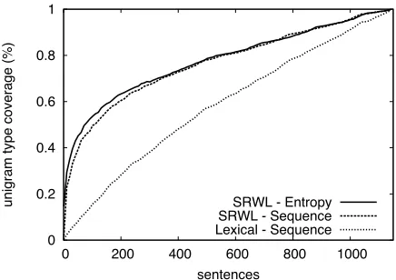
To study one aspect of this phenomena empiri-cally, we examine the rate at which words are first encountered in our training corpus from Section 4, as shown by Figure 3. The first observation is the usefulness of SRWL feature abstraction in gen-eral as we see that when including an entire SRWL from (Pantel and Lin, 2002) whenever the first ele-ment of the list is encountered, we cover the unigram vocabulary much more rapidly. The second observa-tion is that when sentences are presented in the or-der of the average SRWL entropy of their words, this coverage rate is further accelerated. Figure 3 helps explain the recall focused aspect of SRWL abstrac-tion while we rely on hypothesis-driven querying to target interactions for the specific task at hand.
0 0.2 0.4 0.6 0.8 1
0 200 400 600 800 1000
unigram type coverage (%)
sentences
[image:5.612.319.537.59.213.2]SRWL - Entropy SRWL - Sequence Lexical - Sequence
Figure 3: The Impact of SRWL Abstraction and SRWL-driven Querying – The first occurrence of words occur at a much lower rate than the first occurrence of words when abstracted through SRWLs, particularly when sentences are introduced as ranked by average SRWL entropy cal-culated using (Brandts and Franz, 2006).
3.2.3 Aggregating Querying Functions
To combine these two measures, we use the Borda count method of rank aggregation (Young, 1974) to find a consensus between the two querying func-tions without requiring calibration amongst the ac-tual ranking scores. Defining the rank position of an instance byr(x), the Borda count based querying
function is stated by
QBorda= argsort i=1,...,m
[rmargin(xi) +rentropy(xi)]
QBorda selects instances which consider both wide
applicability through rentropy and which focus on
the specific task throughrmargin.
4 Experimental Evaluation
To demonstrate the IFSC protocol on a practical ap-plication, we examine a three-stage pipeline model for entity and relation extraction, where the task is decomposed into sequential stages of segmentation, entity classification, and relation classification (Roth and Small, 2008). Extending the standard classifi-cation task, a pipeline model decomposes the over-all classification into a sequence of D stages such
that each staged = 1, . . . , D has access to the
in-put instance along with the classifications from all previous stages, yˆ(d). Each stage of the pipeline
Φ(d)(x,yˆ(0), . . . ,yˆ(d−1)) → x(d)to learn a
hypoth-esish(d). Once each stage of the pipelined classifier
is learned, predictions are made sequentially, where
ˆ
y=h(x) = *
argmax y0∈Y(d)
f(d)x(d), y0 +D
d=1
Each pipeline stage requires a classifier which makes multiple interdependent predictions based on input from multiple sentence elements x ∈ X1 ×
· · · × Xnx using a structured output space, y(d) ∈ Y1(d) × · · · × Y
(d)
ny. More specifically, segmenta-tion makes a predicsegmenta-tion for each sentence word over Y ∈ {begin, inside, outside} and constraints are enforced between predictions to ensure that an in-sidelabel can only follow abeginlabel. Entity clas-sification begins with the results of the segmenta-tion classifier and classifies each segment intoY ∈ {person, location, organization}. Finally,
rela-tion classificarela-tion labels each predicted entity pair with Y ∈ {located in, work f or, org based in, live in,kill} × {lef t, right}+no relation.
The data used for empirical evaluation was taken from (Roth and Yih, 2004) and consists of 1436 sen-tences, which is split into a 1149 (80%) sentence training set and a 287 (20%) sentence testing set such that all have at least one active relation. SR-WLs are provided by (Pantel and Lin, 2002) and experiments were conducted using a custom graphi-cal user interface (GUI) designed specifigraphi-cally for the IFSC protocol. The learning algorithm used for each stage of the classification task is a regularized vari-ant of the structured Perceptron (Collins, 2002). Re-sources used to perform experiments are available at http://L2R.cs.uiuc.edu/∼cogcomp/.
We extract features in a method similar to (Roth and Small, 2008), except that we do not include gazetteer features in Φ(d)
0 as we will include this
type of external information interactively. Secondly, we use SRWL features as introduced. The segmen-tation features include the word/SRWL itself along with the word/SRWL of three words before and two words after, bigrams of the word/SRWL surround-ing the word, capitalization of the word, and capi-talization of its neighbor on each side. Entity clas-sification uses the segment size, the word/SRWL members within the segment, and a window of two word/SRWL elements on each side. Relation
clas-sification uses the same features as entity classifica-tion along with the entity labels, the length of the entities, and the number of tokens between them.
4.1 Interactive Querying Function
When using the interactive feature space construc-tion protocol for this task, we require a querying function which captures the hypothesis-driven as-pect of instance selection. We observed that basing Qmarginon the relation stage performs best, which
is not surprising given that this stage makes the most mistakes, benefits the most from semantic informa-tion, and also has many features which are similar to features from previous stages. Therefore, we adapt the querying function described by (Roth and Small, 2008) for the relation classification stage and define our margin for the purposes of instance selection as
ρrelation = min i=1,...,ny
fy+(x, i)−fy˙+(x, i)
wherey˙ = argmaxy0∈Y\yfy0(x), the highest
scor-ing class which is not the true label, and Y+ =
Y\no relation.
4.2 Interactive Protocol on Entire Data Set
The first experiments we conduct uses all available training data (i.e. |S| = 1149) to examine the im-provement achieved with a fixed number of IFSC interactions. A single interaction is defined by the expert selecting a lexical element from a sentence presented by the querying function and validating the associated word list. Therefore, it is possible that a single sentence may result in multiple interactions. The results for this experimental setup are sum-marized in Table 1. For each protocol configura-tion, we report F1 measure for all three stages of the pipeline. As our simplest baseline, we first train using the default feature set without any semantic features (Lexical Features). The second baseline is to replace all instances of any lexical element with its SRWL representation as provided by (Pan-tel and Lin, 2002) (Semantic Features). The next two baselines attempt to automatically increase pre-cision by defining each semantic class using only the top fraction of the elements in each SRWL (Pruned
Semantic (top{1/2,1/4})). This pruning procedure
Pruned Pruned 50 interactions
Lexical Semantic Semantic Semantic Interactive Interactive
Features Features (top 1/2) (top 1/4) (select only) (select & validate)
Segmentation 90.23 90.14 90.77 89.71 92.24 93.43
Entity Class. 82.17 83.28 83.93 83.04 85.81 88.76
[image:7.612.71.540.53.138.2]Relation Class. 54.67 55.20 56.34 56.21 59.14 62.08
Table 1: Relative performance of the stated experiments conducted over the entire available dataset. The interactive feature construction protocol outperforms all non-interactive baselines, particularly for later stages of the pipeline while requiring only 50 interactions.
Finally, we consider the interactive feature space construction protocol at two different stages. We first consider the case where 50 interactions are per-formed such that the algorithm assumesW∗ = W, that is, the expert selects features for abstraction, but doesn’t perform validation (Interactive (select
only)). The second experiment performs the entire
protocol, including validation (Interactive (select &
validate)) for 50 interactions. On the relation
ex-traction task, we observe a 13.6% relative improve-ment over the lexical model and a 10.2% relative im-provement over the best SRWL baseline F1 score.
4.3 Examination of the Querying Function
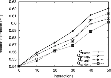
As stated in section 3.2, an appropriate querying function presents sentences which will result in the expert selecting features from that example and for which the resulting interactions will result in a large performance increase. The former is difficult to model, as it is dependent on properties of the sen-tence (such as length), will differ from user to user, and anecdotally is negligibly different for the three querying functions for earlier interactions. How-ever, we are able to measure the performance im-provement of interactions associated with different querying functions. For our second experiment, we evaluate the relative performance of the three query-ing functions defined after every ten interactions in terms of the F1 measure for relation extraction. The results of this experiment are shown in figure 4, where we first see that theQrandom generally leads
to the least useful interactions. Secondly, while Qentropy performs well early, Qmargin works
bet-ter as more inbet-teractions are performed. Finally, we also observe that QBorda exceeds the performance
envelope of the two constituent querying functions.
0.54 0.55 0.56 0.57 0.58 0.59 0.6 0.61 0.62 0.63
0 10 20 30 40 50
relation extraction (F1)
interactions QBorda Qentropy Qmargin Qrandom
Figure 4: Relative performance of interactions generated through the respective querying functions. We see that
Qentropy performs well for a small number of interac-tions, Qmargin performs well as more interactions are performed andQBordaoutperforms both consistently.
4.4 Robustness to Reduced Annotation
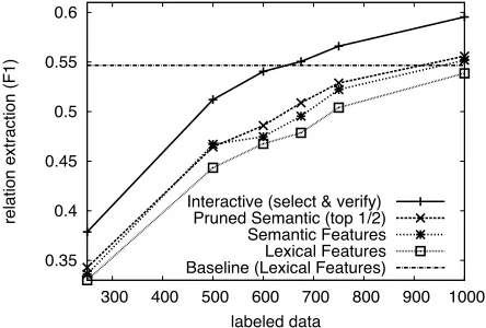
The third set of experiments consider the relative performance of the configurations from the first set of experiments as the amount of available training data is reduced. To study this scenario, we per-form the same set of experiments with 50 interac-tions while varying the size of the training set (e.g. |S| = {250,500,600,675,750,1000}),
[image:7.612.317.536.212.365.2]interpo-lation of the performance at 600 and 675 labeled in-stances implies that we achieve a performance level comparable to training on all of the data of the base-line learner while about 55% of the labeled data is observed at random. Furthermore, as more labeled data is introduced, the performance continues to im-prove with only 50 interactions. This supports the hypothesis that a good representation is often more important than additional training data, even when the data is carefully selected.
0.35 0.4 0.45 0.5 0.55 0.6
300 400 500 600 700 800 900 1000
relation extraction (F1)
labeled data Interactive (select & verify)
[image:8.612.73.295.211.361.2]Pruned Semantic (top 1/2) Semantic Features Lexical Features Baseline (Lexical Features)
Figure 5: Relative performance of several baseline al-gorithm configurations and the interactive feature space construction protocol with variable labeled dataset sizes. The interactive protocol outperforms other baseline meth-ods in all cases. Furthermore, the interactive protocol (In-teractive)outperforms the baseline lexical system (Base-line) trained on all 1149 sentences even when trained with a significantly smaller subset of labeled data.
5 Related Work
There has been significant recent work on designing learning algorithms which attempt to reduce annota-tion requirements through a more sophisticated an-notation method. These methods allow the annota-tor to directly specify information about the feature space in addition to providing labels, which is then incorporated into the learning algorithm (Huang and Mitchell, 2006; Raghavan and Allan, 2007; Zaidan et al., 2007; Druck et al., 2008; Zaidan and Eisner, 2008). Additionally, there has been recent work us-ing explanation-based learnus-ing techniques to encode a more expressive feature space (Lim et al., 2007). Amongst these works, the only interactive learning protocol is (Raghavan and Allan, 2007) where
in-stances are presented to an expert and features are labeled which are then emphasized by the learning algorithm. Thus, in this case, although additional information is provided the feature space itself re-mains static. To the best of our knowledge, this is the first work that interactively modifies the feature space by abstracting the FGFs.
6 Conclusions and Future Work
This work introduces the interactive feature space constructionprotocol, where the learning algorithm selects examples for which the feature space is be-lieved to be deficient and uses existing semantic resources in coordination with a domain expert to abstract lexical features with their SRWL names. While the power of SRWL abstraction in terms of sample complexity is evident, incorporating this formation is fraught with pitfalls regarding the in-troduction of additional ambiguity. This interactive protocol finds examples for which the domain ex-pert will recognize promising semantic abstractions and for which those semantic abstraction will signif-icantly improve the performance of the learner. We demonstrate the effectiveness of this protocol on a named entity and relation extraction system.
As a relatively new direction, there are many possibilities for future work. The most immedi-ate task is effectively quantifying interaction costs with a user study, including the impact of includ-ing users with varyinclud-ing levels of expertise. Recent work on modeling the costs of the active learn-ing protocol (Settles et al., 2009; Haertel et al., 2009) provides some insight on modeling costs as-sociated with interactive learning protocols. A sec-ond potentially interesting direction would be to incorporate other semantic resources such as lexi-cal patterns (Hearst, 1992) or Wikipedia-generated gazetteers (Toral and Mu˜noz, 2006).
Acknowledgments
References
Avrim Blum. 1992. Learning boolean functions in an infinite attribute space. Machine Learning, 9(4):373– 386.
Lois Boggess, Rajeev Agarwal, and Ron Davis. 1991. Disambiguation of prepositional phrases in automat-ically labelled technical text. In Proceedings of the National Conference on Artificial Intelligence (AAAI), pages 155–159.
Thorsten Brandts and Alex Franz. 2006. Web 1T 5-gram Version 1.
David Cohn, Les Atlas, and Richard Ladner. 1994. Im-proving generalization with active learning. Machine Learning, 15(2):201–222.
Michael Collins. 2002. Discriminative training methods for hidden markov models: Theory and experiments with perceptron algorithms. InProc. of the Conference on Empirical Methods for Natural Language Process-ing (EMNLP), pages 1–8.
Gregory Druck, Gideon Mann, and Andrew McCallum. 2008. Learning from labeled features using general-ization expectation criteria. InProc. of International Conference on Research and Development in Informa-tion Retrieval (SIGIR), pages 595–602.
Christiane Fellbaum. 1998. WordNet: An Electronic Lexical Database. MIT Press.
Robbie Haertel, Kevin D. Seppi, Eric K. Ringger, and James L. Carroll. 2009. Return on investment for active learning. InNIPS Workshop on Cost Sensitive Learning.
Marti A. Hearst. 1992. Automatic acquisition of hy-ponyms from large text corpora. In Proc. the In-ternational Conference on Computational Linguistics (COLING), pages 539–545.
Yifen Huang and Tom M. Mitchell. 2006. Text clustering with extended user feedback. InProc. of International Conference on Research and Development in Informa-tion Retrieval (SIGIR), pages 413–420.
Xin Li and Dan Roth. 2005. Learning question clas-sifiers: The role of semantic information. Journal of Natural Language Engineering, 11(4).
Siau Hong Lim, Li-Lun Wang, and Gerald DeJong. 2007. Explanation-based feature construction. In Proc. of the International Joint Conference on Artificial Intelli-gence (IJCAI), pages 931–936.
Scott Miller, Jethran Guinness, and Alex Zamanian. 2004. Name tagging with word clusters and discrimi-native training. InProc. of the Annual Meeting of the North American Association of Computational Lin-guistics (NAACL), pages 337–342.
Patrick Pantel and Dekang Lin. 2002. Discovering word senses from text. InProc. of the International Con-ference on Knowledge Discovery and Data Mining (KDD), pages 613–619.
Hema Raghavan and James Allan. 2007. An interactive algorithm for asking and incorporating feature feed-back into support vector machines. InProc. of Inter-national Conference on Research and Development in Information Retrieval (SIGIR), pages 79–86.
Dan Roth and Kevin Small. 2008. Active learning for pipeline models. InProceedings of the National Con-ference on Artificial Intelligence (AAAI), pages 683– 688.
Dan Roth and Wen-Tau Yih. 2004. A linear program-ming formulation for global inference in natural lan-guage tasks. In Proc. of the Annual Conference on Computational Natural Language Learning (CoNLL), pages 1–8.
Burr Settles, Mark Craven, and Lewis Friedland. 2009. Active learning with real annotation costs. InNIPS Workshop on Cost Sensitive Learning.
Simon Tong and Daphne Koller. 2001. Support vec-tor machine active learning with applications to text classification.Journal of Machine Learning Research, 2:45–66.
Antonio Toral and Rafael Mu˜noz. 2006. A proposal to automatically build and maintain gazetteers using wikipedia. In Proc. of the Annual Meeting of the European Association of Computational Linguistics (EACL), pages 56–61.
H. Peyton Young. 1974. An axiomatization of borda’s rule. Journal of Economic Theory, 9(1):43–52. Omar F. Zaidan and Jason Eisner. 2008. Modeling
anno-tators: A generative approach to learning from annota-tor rationales. InProc. of the Conference on Empirical Methods for Natural Language Processing (EMNLP), pages 31–40.