Uncertainty Detection as Approximate Max-Margin Sequence Labelling
Oscar T¨ackstr¨omSICS / Uppsala University Kista / Uppsala, Sweden
Gunnar Eriksson SICS Kista, Sweden [email protected]
Sumithra Velupillai DSV, Stockholm University
Kista, Sweden [email protected]
Hercules Dalianis DSV, Stockholm University
Kista, Sweden [email protected]
Martin Hassel DSV, Stockholm University
Kista, Sweden [email protected]
Jussi Karlgren SICS Kista, Sweden [email protected]
Abstract
This paper reports experiments for the CoNLL-2010 shared task on learning to detect hedges and their scope in natu-ral language text. We have addressed the experimental tasks as supervised lin-ear maximum margin prediction prob-lems. For sentence level hedge detection
in the biological domain we use an L1
-regularised binary support vector machine, while for sentence level weasel detection
in the Wikipedia domain, we use anL2
-regularised approach. We model the in-sentence uncertainty cue and scope
de-tection task as anL2-regularised
approxi-mate maximum margin sequence labelling
problem, using the BIO-encoding. In
ad-dition to surface level features, we use a variety of linguistic features based on a functional dependency analysis. A greedy forward selection strategy is used in ex-ploring the large set of potential features. Our official results for Task 1 for the
bio-logical domain are 85.2F1-score, for the
Wikipedia set 55.4F1-score. For Task 2,
our official results are 2.1 for the entire task with a score of 62.5 for cue detec-tion. After resolving errors and final bugs, our final results are for Task 1, biologi-cal: 86.0, Wikipedia: 58.2; Task 2, scopes: 39.6 and cues: 78.5.
1 Introduction
This paper reports experiments to detect uncer-tainty in text. The experiments are part of the two shared tasks given by CoNLL-2010 (Farkas et al., 2010). The first task is to identify uncertain sen-tences; the second task is to detect the cue phrase which makes the sentence uncertain and to mark its scope or span in the sentence.
Uncertainty as a target category needs to be ad-dressed with some care. Sentences, utterances, statements are not uncertain – their producer, the speaker or author, is. Statements may explicitly indicate this uncertainty, employing several differ-ent linguistic and textual mechanisms to encode the speaker’s attitude with respect to the verac-ity of an utterance. The absence of such markers does not necessarily indicate certainty – the oppo-sition between certain and uncertain is not clearly demarkable, but more of a dimensional measure. Uncertainty on the part of the speaker may be dif-ficult to differentiate from a certain assessment of
an uncertain situation, It is unclear whether this
specimen is an X or a Yvs.The difference between X and Y is unclear.
In this task, the basis for identifying uncertainty
in utterances is almost entirely lexical. Hedges,
the main target of this experiment, are an estab-lished category in lexical grammar analyses - see e.g. Quirk et al. (1985), for examples of English language constructions. Most languages use vari-ous verbal markers or modifiers for indicating the speaker’s beliefs in what is being said, most proto-typically using conditional or optative verb forms,
Six Parisiens seraient morts, or auxiliaries, This mushroom may be edible, but aspectual markers may also be recruited for this purpose, more
indi-rectly,I’m hoping you will helpvs.I hope you will
help;Do you want to see me nowvs.Did you want to see me now. Besides verbs, there are classes of terms that through their presence, typically in an adverbial role, in an utterance make explicit
its tentativeness: possibly, perhaps... and more
complex constructionswith some reservation,
es-pecially such that explicitly mention the speaker
and the speaker’s beliefs or doubts,I suspect that
X.
Weasels, the other target of this experiment, on the other hand, do not indicate uncertainty.
Weasels are employed when speakers attempt to convince the listener of something they most likely are certain of themselves, by anchoring the truth-fulness of the utterance to some outside fact or
au-thority (Most linguists believe in the existence of
an autonomous linguistic processing component), but where the authority in question is so unspecific as not to be verifiable when scrutinised.
We address both CoNLL-2010 shared tasks (Farkas et al., 2010). The first, detecting uncer-tain information on a sentence level, we solve by
using an L1-regularised support vector machine
with hinge loss for the biological domain, and
anL2-regularised maximum margin model for the
Wikipedia domain. The second task, resolution of in-sentence scopes of hedge cues, we approach as
an approximate L2-regularized maximum margin
structured prediction problem. Our official results
for Task 1 for the biological domain are 85.2F1
-score, for the Wikipedia set 55.4 F1-score. For
Task 2, our official results were 2.1 for the entire task with a score of 62.5 for cue detection. After resolving errors and unfortunate bugs, our final re-sults are for Task 1, biological: 86.0, Wikipedia: 58.2; Task 2: 39.6 and 78.5 for cues.
2 Detecting Sentence Level Uncertainty
On the sentence level, word- and lemma-based features have been shown to be useful for uncer-tainty detection (see e.g. Light et al. (2004), Med-lock and Briscoe (2007), MedMed-lock (2008), and Szarvas (2008)). Medlock (2008) and Szarvas (2008) employ probabilistic, weakly supervised methods, where in the former, a stemmed single term and bigram representation achieved best re-sults (0.82 BEP), and in the latter, a more complex n-gram feature selection procedure was applied using a Maximum Entropy classifier, achieving best results when adding reliable keywords from an external hedge keyword dictionary (0.85 BEP,
85.08F1-score on biomedical articles). More
lin-guistically motivated features are used by Kil-icoglu and Bergler (2008), such as negated
“un-hedging” verbs and nouns and that preceded by
epistemic verbs and nouns. On the fruit-fly dataset (Medlock and Briscoe, 2007) they achieve 0.85 BEP, and on the BMC dataset (Szarvas, 2008) they achieve 0.82 BEP. Light et al. (2004) also found that most of the uncertain sentences appeared to-wards the end of the abstract, indicating that the position of an uncertain sentence might be a
use-ful feature.
Ganter and Strube (2009) consider weasel tags in Wikipedia articles as hedge cues, and achieve results of 0.70 BEP using word- and distance based features on a test set automatically derived from Wikipedia, and 0.69 BEP on a manually an-notated test set using syntactic patterns as fea-tures. These results suggest that syntactic features are useful for identifying weasels that ought to be tagged. However, evaluation is performed on bal-anced test sets, which gives a higher baseline.
2.1 Learning and Optimization Framework
A guiding principle in our approach to this shared task has been to focus on highly computationally efficient models, both in terms of training and pre-diction times. Although kernel based non-linear separators may sometimes obtain better predic-tion performance, compared to linear models, the speed penalty at prediction time is often substan-tial, since the number of support patterns often grows linearly with the size of the training set. We therefore restrict ourselves to linear models, but allow for a restricted family of explicit non-linear mappings by feature combinations.
For sentence level hedge detection in the
bio-logical domain, we employ anL1-regularised
sup-port vector machine with hinge loss, as provided by the library implemented by Fan et al. (2008), while for weasel detection in the Wikipedia
do-main, we instead use theL2-regularised maximum
margin model described in more detail in section 3.1. In both cases, we approximately optimise the
F1-measure by weighting each class by the inverse
of its proportion in the training data.
The reason for usingL1-regularisation in the
bi-ological domain is that the annotation is heavily biased towards a rather small number of lexical cues, making most of the potential surface features irrelevant. The Wikipedia weasel annotation, on the other hand, is much more noisy and less de-termined by specific lexical markers. Regularising
with respect to theL1-norm is known to give
pref-erence to sparse models and for the special case of logistic regression, Ng (2004) proved that the sample complexity grows only logarithmically in the number of irrelevant features, instead of
lin-early as when regularising with respect to theL2
-norm. Our preliminary experiments indicated that
L1-regularisation is superior to L2-regularisation
the Wikipedia domain.
2.2 Feature Definitions
The asymmetric relationship between certain and uncertain sentences becomes evident when one tries to learn this distinction based on surface level
cues. While theUNCERTAINcategory is to a large
extent explicitly anchored in lexical markers, the CERTAINcategory is more or less defined
implic-itly as the complement of the UNCERTAIN
cate-gory. To handle this situation, we use a bias
fea-ture to model the weight of theCERTAINcategory,
while explicit features are used to model the
UN-CERTAINcategory.
The following list describes the feature tem-plates explored for sentence level uncertainty de-tection. Some features are based on a linguistic analysis by the Connexor Functional Dependency (FDG) parser (Tapanainen and J¨arvinen, 1997).
SENLEN Preliminary experiments indicated that taking sen-tence length into account is beneficial. We incorporate this by using three different bias terms, according to the length (in tokens) of the sentences. This feature takes the following values:S<18≤M≤32<L.
DOCPT Document part, e.g.,TITLE,ABSTRACTandBODY TEXT, allowing for different models for different docu-ment parts.
TOKEN, LEMMA Tokens in most cases equals words, but may in some special cases also be multiword units, e.g.
of course, as defined by the FDG tokenisation. Lemmas are base forms of words, with some special features introduced for numeric tokens, e.g., year, short number, and long number.
QUANT Syntactic function of a noun phrase with a quanti-fier head (at leastsome of the isoformsare conserved between mouse and humans), or a modifying quantifier (Recently,many investigatorshave been interested in the study on eosinophil biology).
HEAD, DEPREL Functional dependency head of the token, and the type of dependency relation between the head and the token, respectively.
SYN Phrase-level and clause-level syntactic functions of a word.
MORPH Part-of-speech and morphological traits of a word. Each feature template defines a set of features when applied to data. The TOKEN, LEMMA,
QUANT, HEAD, DEPREL templates yield
single-ton sets of features for each token, while the SYN
and MORPH templates extends to sets consisting
of several features for each token. A sentence is represented as the union of all active token level
features and the SENLEN and DOCPT, if active.
In addition to the linear combination of concrete
features, we allow combined features by the Carte-sian product of the feature set extensions of two or more feature templates.
2.3 Feature Template Selection
Although regularised maximum margin models often cope well even in the presence of irrelevant features, it is a good idea to search the large set of potential features for an optimal subset.
In order to make this search feasible we make two simplifications. First, we do not explore the full set of individual features, but instead the set of feature templates, as defined above. Second, we perform a greedy search in which we iteratively add the feature template that gives the largest per-formance improvement, when added to the cur-rent optimal set of templates. The performance of a feature set for sentence level detection is
mea-sured as the mean F1-score, with respect to the
UNCERTAIN class, minus one standard deviation – the mean and standard deviation are computed by three fold cross-validation on the training set. We subtract one standard deviation from the mean in order to promote stable solutions over unstable ones.
Of course, these simplifications do not come for free. The solution of the optimisation problem might be quite unstable with respect to the optimal hyper-parameters of the learning algorithm, which in turn may depend on the feature set used. This risk could be reduced by conducting a more thor-ough parameter search for each candidate feature set, however, this was simply too time consuming for the present work. A further risk of using for-ward selection is that feature interactions are ig-nored. This issue is handled better with backward elimination, but that is also more time consuming. The full set of explored feature templates is too large to be listed here; instead we list the features selected in each iteration of the search, together with their corresponding scores, in Table 1.
3 Detecting In-sentence Uncertainty
cur-Task Template set DevF1 TestF1
Bio
SENLEN -
-∪LEMMA 88.9 (.25) 78.79
∪LEMMABI 90.3 (.19) 85.86
∪LEMMA⊗QUANT 90.3 (.07) 85.97
Wiki ∪SENTOKENLEN ⊗DOCPT 59.0 (.76)- 60.12
-∪TOKENBI⊗SENLEN 59.9 (.09) 58.26
Table 1: Top feature templates for sentence level hedge and weasel detection.
rent lemma as features) and 82.82 F-score (using a Support Vector Machine classifier and a complex feature set including keyword and dependency re-lation information), respectively. On the task of automatic scope resolution, best results are re-ported as 59.66 (F-score) and 61.13 (accuracy), respectively, on the full paper subset. ¨Ozg¨ur and Radev (2009) use a rule-based method for this sub-task, while Morante and Daelemans (2009) use three different classifiers as input to a CRF-based meta-learner, with a complex set of features, in-cluding hedge cue information, current and sur-rounding token information, distance information and location information.
3.1 Learning and Optimisation Framework
In recent years, a wide range of different ap-proaches to general structured prediction prob-lems, of which sequence labelling is a special case, have been suggested. Among others, Con-ditional Random Fields (Lafferty et al., 2001), Max-Margin Markov Networks (Taskar et al., 2003), and Structured Support Vector Machines (Tsochantaridis et al., 2005). A drawback of these approaches is that they are all quite com-putationally demanding. As an alternative, we propose a much more computationally lenient ap-proach based on the regularised margin-rescaling formulation of Taskar et al. (2003), which we in-stead optimise by stochastic subgradient descent as suggested by Ratliff et al. (2007). In addi-tion we only perform approximate decoding, us-ing beam search, which allows arbitrary complex joint feature maps to be employed, without sacri-ficing speed.
3.1.1 Technical Details
LetX denote the pattern set and letY denote the
set of structured labels. Let A denote the set of
atomic labels and let each labely ∈ Y consist of
an indexed sequence of atomic labelsyi ∈ A.
De-note byYx ⊆ Y the set of possible label
assign-ments to patternx ∈ X and byyx ∈ Yx its
cor-rect label. In the specific case of BIO-sequence
labelling, A = {BEGIN,INSIDE,OUTSIDE} and
Yx=A|x|, where|x|is the length of the sequence
x∈ X.
A structured classification problem amounts to learning a mapping from patterns to labels,
f : X 7→ Y, such that the expected loss
EX ×Y[∆(yx, f(x))]is minimised. The prediction
loss, ∆ : Y × Y 7→ <+, measures the loss of
predicting label y = f(x) when the correct
la-bel is yx, with ∆(yx, yx) = 0. Here we assume
the Hamming loss, ∆H(y, y0) = P|i=1y| δ(yi, y0i),
whereδ(yi, y0i) = 1ifyi 6=yi0and0otherwise.
The idea of the margin-rescaling approach is to
let thestructured marginbetween the correct label
yxand a hypothesisy ∈ Yxscale linearly with the
prediction loss∆(yx, y)(Taskar et al., 2003). The
structured margin is defined in terms of a score
functionS : X × Y 7→ <, in our case the linear
score functionS(x, y) =wTΦ(x, y), wherew∈
<mis a vector of parameters andΦ :X ×Y 7→ <m
is a joint feature function. The learning problem
then amounts to finding parameters w such that
S(x, yx) ≥ S(x, y) + ∆(yx, y) for ally ∈ Yx\
{yx}over the training dataD. In other words, we
want the score of the correct label to be higher than
the scoreplus the loss, of all other labels, for each
instance. In order to balance margin maximisation
and margin violation, we add theL2-regularisation
termkwk2.
By making use of theloss augmenteddecoding
function
f∆(x, yx) = argmax y∈Yx
[S(x, y) + ∆(yx, y)], (1)
we get the following regularised risk functional:
Qλ,D(w) = |D|
X
i=1
S∆(x(i), yx(i)) +
λ
2kwk2, (2)
where
S∆(x, yx) = max y∈Yx
[S(x, y) + ∆(yx, y)]−S(x, yx) (3) We optimise (2) by stochastic approximate
subgra-dient descent with step size sequence[η0/
√
t]∞t=1
(Ratliff et al., 2007). The initial step size η0
and the regularisation factor λ are data
This framework is highly efficient both at learn-ing and prediction time. Trainlearn-ing cues and scopes on the biological data, takes about a minute, while prediction times are in the order of seconds, using a Java based implementation on a standard laptop; the absolute majority of that time is spent on read-ing and extractread-ing features from an inefficient
in-ternalJSON-based format.
3.1.2 Hashed Feature Functions
Joint feature functions enable encoding of depen-dencies between labels and relations between pat-tern and label. Most feature templates are fined based on input only, while some are de-fined with respect to output features as well. Let Ψ(x, y1:i−1, i)∈ <mdenote the joint feature
func-tion corresponding to the applicafunc-tion of all active
feature templates to pattern x ∈ X and partially
decoded label y1:i−1 ∈ Ai−1 when decoding at
position i. The feature mapping used in scoring
candidate label yi ∈ A is then computed as the
Cartesian product Φ(x, y, i) = Ψ(x, y1:i−1, i) ⊗
Λ(yi), whereΛ(yi)∈ <mis a unique unitary
fea-ture vector representation of labelyi. The feature
representation for a complete sequence x and its
associated labelyis then computed as
Φ(x, y) =
|x|
X
i=1
Φ(x, y, i)
When employing joint feature functions and com-bined features, the number of unique features may grow very large. This is a problem when the amount of internal memory is limited. Feature hashing, as described by Weinberger et al. (2009), is a simple trick to circumvent this problem. As-sume that we have an original feature function
φ : X × Y 7→ <m, where m might be
arbitrar-ily large. Leth :N+ 7→ [1, n]be a hash function
and leth−1(i)⊆[1, m]be the set of integers such
thatj ∈ h−1(i) iffh(j) = i. We now use this
hash function to map the index of each feature in
φ(x, y) to its corresponding index in Φ(x, y), as
Φi(x, y) =Pj∈h−1(i)φj(x, y). The features inΦ
are thus unions of multisets of features inφ. Given
a hash function with good collision properties, we can expect that the subset of features mapped to
any index inΦ(x, y)is small and composed of
ele-ments drawn at random fromφ(x, y). Weinberger
et al. (2009) contains proofs of bounds on these
distributions. Furthermore, by using a k-valued
hash functionh:Nk7→[1, n], the Cartesian
prod-uct ofkfeature sets can be computed much more
efficiently, compared to using a dictionary.
3.2 Position Based Feature Definitions
For in-sentence cue and scope prediction we make use of the same token level feature templates as for sentence level detection. An additional level of expressivity is added in that each token level template is associated with a token position. A template is addressed either relative to the token currently being decoded, or by the dependency arc of a token, which in turn is addressed by a relative position. The addressing can be either to a single position, or a range of positions. Feature templates may further be defined with respect to features of the input pattern, the token level labels predicted so far, or with respect to combinations of input and label features. Joint features, just as complex feature combinations, are created by forming the Cartesian product of an input feature set and a la-bel feature set.
The feature templates are instantiated by pre-fixing the template name to each member of the feature set. To exemplify, the single position
tem-plate TOKENi, given that the token currently
be-ing decoded at position i issuggests, is
instanti-ated as the singleton set {TOKENi = suggests}.
The range template TOKENi,i+1, given that the
current token is suggests and the next token is
that, is instantiated as the set {TOKENi,i+1 =
suggests,TOKENi,i+1 = that}; i.e. each member
of the set is prefixed by the range template name. In addition to the token level templates used for sentence level prediction, the following templates were explored:
LABEL Label predicted so far at the addressed position(s).
HEAD.X An arbitrary feature, X, addressed by follow-ing the dependency arc(s) from the addressed posi-tion(s). For example, HEAD.LEMMAicorresponds to
the lemma found by looking at the dependency head of the current token.
CUE, CUESCOPE Whether the token(s) addressed is re-spectively, a cue marker, or within the syntactic scope of the current cue, following the definition of scope provided by Vincze et al. (2008).
3.3 Feature Template Selection
The scoring measures used in the search for cue and scope detection features differ. In order to match the official scoring measure for cue
de-tection, we optimise the F1-score of labels
cor-responding to cue tags, i.e. we treat the BEGIN
andINSIDEcue tags as an equivalence class. The official scoring measure for scope prediction, on the other hand, corresponds to the exact match of scope boundaries. Unfortunately using exact match performance turned out to be not very well suited for use in greedy forward selection. This is because before a sufficient per token accuracy has been reached, and even when it has, the ex-act match score may fluctuate wildly. Therefore, as a substitute, we instead guide the search by to-ken level accuracy. This discrepancy between the search criterion and the official scoring metric is unfortunate.
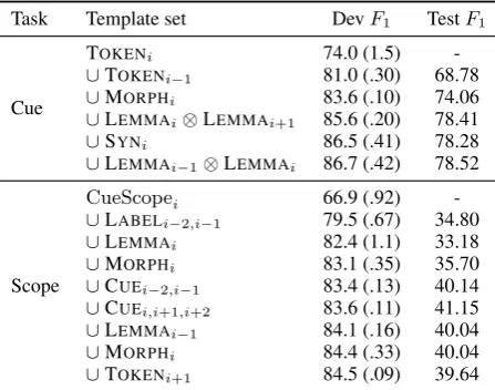
Again, when taking into account position ad-dressing, joint features and combined features, the complete set of explored templates is too large to fit in the current experiment. The selected features together with their corresponding scores are found in Table 2.
Task Template set DevF1 TestF1
Cue
TOKENi 74.0 (1.5)
-∪TOKENi−1 81.0 (.30) 68.78
∪MORPHi 83.6 (.10) 74.06
∪LEMMAi⊗LEMMAi+1 85.6 (.20) 78.41
∪SYNi 86.5 (.41) 78.28
∪LEMMAi−1⊗LEMMAi 86.7 (.42) 78.52
Scope
CueScopei 66.9 (.92)
-∪LABELi−2,i−1 79.5 (.67) 34.80
∪LEMMAi 82.4 (1.1) 33.18
∪MORPHi 83.1 (.35) 35.70
∪CUEi−2,i−1 83.4 (.13) 40.14
∪CUEi,i+1,i+2 83.6 (.11) 41.15
∪LEMMAi−1 84.1 (.16) 40.04
∪MORPHi 84.4 (.33) 40.04
[image:6.595.73.297.401.577.2]∪TOKENi+1 84.5 (.09) 39.64
Table 2: Top feature templates for in-sentence de-tection of hedge cues and scopes.
4 Discussion
Our finalF1-score results for the corrected system
are, in Task 1 for the biological domain 85.97, for the Wikipedia domain 58.25; for Task 2, our re-sults are 39.64 for the entire task with a score of 78.52 for cue detection.
Any gold standard-based shared experiment un-avoidably invites discussion on the reliability of
the gold standard. It is easy to find borderline ex-amples in the evaluation corpus, e.g. sentences that may just as well be labeled “certain” rather than “uncertain”. This gives an indication of the true complexity of assessing the hidden variable of uncertainty and coercing it to a binary judgment rather than a dimensional one. It is unlikely that everyone will agree on a binary judgment every time.
To improve experimental results and the gen-eralisability of the results for the task of detect-ing uncertain information on a sentence level, we would need to break reliance on the purely lexical
cues. For instance, we now have identified
possi-bleandputativeas markers for uncertainty, but in
many instances they are not (Finally, we wish to
ensure that others can use and evaluate the GREC as simply as possible). This would be avoidable through either a deeper analysis of the sentence
to note thatpossiblein this case does not modify
anything of substance in the sentence, or alterna-tively through a multi-word term preprocessor to
identifyas simply as possibleas an analysis unit.
In the Wikipedia experiment, where the
objec-tive is to identifyweaselphrases, the judicious
en-coding of quantifiers such as “some of the most
well-known researchers say that X” would be
likely to identify the sought-for sentences when the quantified NP is in subject position. In our experiment we find that our dependency analysis did not distinguish between the various syntactic roles of quantified NPs. As a result, we marked several sentences with a quantifier as a “weasel” sentence, even where the quantified NP was in a non-subject role – leading to overly many weasel sentences. An example is given in Table 3.
and established challenge for NLP systems in gen-eral.
In the task of detecting in-sentence uncertainty – identification of hedge cues and their scopes – we find that an evaluation method based on ex-act match of a token sequence is overly unforgiv-ing. There are many cases where the marginal to-kens of a sequence are less than central or irrele-vant for the understanding of the hedge cue and its scope: moving the boundary by one position over an uninteresting token may completely invalidate an otherwise arguably correct analysis. A token-by-token scoring would be a more functional eval-uation criterion, or perhaps a fuzzy match, allow-ing for a certain amount of erroneous characters.
For our experiments, this has posed some
chal-lenges. While we model the in-sentence
un-certainty detection as a sequence labelling
prob-lem in the BIO-representation (BEGIN, INSIDE,
OUTSIDE), the provided corpus uses an XML-representation. Moreover, the official scoring tool
requires that the predictions are well formedXML,
necessitating a conversion fromXMLtoBIO prior
to training and fromBIOtoXMLafter prediction.
Consistent tokenisation is important, but the syn-tactic analysis components used by us distorted the original tokenisation and restoring the exact same token sequence proved problematic.
Conversion fromBIOtoXMLis straightforward
for cues, while some care must be taken when an-notating scopes, since erroneous scope predictions
may result in malformedXML. When adding the
scope annotation, we use a stack based algorithm. For each sentence, we simultaneously traverse the scope-sequence corresponding to each cue, left to right, token by token. The stack is used to en-sure that scopes are either separated or nested and an additional restriction ensures that scopes may never start or end inside a cue. In case the al-gorithm fails to place a scope according to these restrictions, we fall back and let the scope cover the whole sentence. Several of the more frequent errors in our analyses are scoping errors, many likely to do with the fallback solution. Our analy-sis quite frequently fails also to assign the subject of a sentence to the scope of a hedging verb. Ta-ble 3 shows one example each of these errors – overextended scope and missing subject.
Unfortunately, the tokenisation output by our analysis components is not always consistent with the tokenisation assumed by the BioScope
annota-tion. A post-processing step was therefore added in which each, possibly complex, token in the
pre-dictedBIO-sequence is heuristically mapped to its
corresponding position in theXMLstructure. This
post-processing is not perfect and scopes and cues at non-word token boundaries, such as parenthe-ses, are quite often misplaced with respect to the BioScope annotation. Table 3 gives one example which is scored “erroneous” since the token “(63)” is in scope, where the “correct” solution has it out-side the scope. These errors are not important to address, but are quite frequent in our results – ap-proximately 80 errors are of this type.
To achieve more general and effective methods to detect uncertainty in an argument, we should note that uncertainty is signalled in a text through many mechanisms, and that the purely lexical and explicit signal found through the present experi-ments in hedge identification is effective and use-ful, but will not catch everything we might want to find. Lexical approaches are also domain depen-dent. For instance, Szarvas (2008) and Morante and Daelemans (2009) report loss in performance, when applying the same methods developed on bi-ological data, on clinical text. Using the systems developed for scientific text elsewhere poses a mi-gration challenge. It would be desirable both to automatically learn a hedging lexicon from a gen-eral seed set and to have features on a higher level of abstraction.
Our main result is that casting this task as a se-quence labelling problem affords us the possibility to combine linguistic analyses with a highly effi-cient implementation of a max-margin prediction algorithm. Our framework processes the data sets in minutes for training and seconds for prediction on a standard personal computer.
5 Acknowledgements
The authors would like to thank Joakim Nivre for feedback in earlier stages of this work. This work was funded by The Swedish National Grad-uate School of Language Technology and by the Swedish Research Council.
References
Rong-En Fan, Kai-Wei Chang, Cho-Jui Hsieh, Xiang-Rui Wang, and Chih-Jen Lin. 2008. LIBLINEAR: A library for large linear classification. Journal of Machine Learn-ing Research, 9:1871–1874.
Neg + certain However, how IFN-γand IL-4 inhibit IL-17 production isnotyetknown.
Neg + certain The mechanism by which Tregs preserve peripheral tolerance is stillnotentirelyclear. “some”: not weasel Tourist folks usually visit this peaceful paradise to enjoysome leisurenonsubj.
“some”: weasel Somesubjsuggest that the origin of music likely stems from naturally occurring sounds and rhythms.
Prediction dRas85DV12<xcope .1><cue .1>may</cue>be more potent than dEGFRλbecause dRas85DV12 can activate endogenous PI3K signaling [16]</xcope>.
Gold standard dRas85DV12<xcope .1><cue .1>may</cue>be more potent than dEGFRλ</xcope>because dRas85DV12 can activate endogenous PI3K signaling [16].
Prediction However, the precise molecular mechanisms of Stat3-mediated expression of RORγt <xcope .1>are still<cue .1>unclear</cue></xcope>.
Gold standard However,<xcope .1>the precise molecular mechanisms of Stat3-mediated expression of RORγt are still<cue .1>unclear</cue></xcope>.
Prediction Interestingly, Foxp3<xcope .1><cue .1>may</cue>inhibit RORγt
activity on its target genes, at least in par,t through direct interaction with RORγt (63)</xcope>. Gold standard Interestingly, Foxp3<xcope .1><cue .1>may</cue>inhibit RORt
activity on its target genes, at least in par,t through direct interaction with RORt</xcope>(63). Table 3: Examples of erroneous analyses.
Csirik, and Gy¨orgy Szarvas. 2010. The CoNLL-2010 Shared Task: Learning to Detect Hedges and their Scope in Natural Language Text. In Proceedings of the 14th Conference on Computational Natural Language Learn-ing (CoNLL-2010): Shared Task, pages 1–12, Uppsala, Sweden, July. Association for Computational Linguistics. Viola Ganter and Michael Strube. 2009. Finding hedges by chasing weasels: hedge detection using Wikipedia tags and shallow linguistic features. InACL-IJCNLP ’09: Pro-ceedings of the ACL-IJCNLP 2009 Conference Short Pa-pers, Morristown, NJ, USA. Association for Computa-tional Linguistics.
Halil Kilicoglu and Sabine Bergler. 2008. Recognizing spec-ulative language in biomedical research articles: a linguis-tically motivated perspective.BMC Bioinformatics, 9. John D. Lafferty, Andrew McCallum, and Fernando C. N.
Pereira. 2001. Conditional random fields: Probabilis-tic models for segmenting and labeling sequence data. In
Proc. 18th Int. Conf. on Machine Learning. Morgan Kauf-mann Publishers.
Marc Light, Xin Ying Qiu, and Padmini Srinivasan. 2004. The language of bioscience: Facts, speculations, and state-ments in between. In Lynette Hirschman and James Pustejovsky, editors, HLT-NAACL 2004 Workshop: Bi-oLINK 2004, Linking Biological Literature, Ontologies and Databases, Boston, USA. ACL.
Ben Medlock and Ted Briscoe. 2007. Weakly supervised learning for hedge classification in scientific literature. In
Proceedings of the 45th Annual Meeting of the Associa-tion of ComputaAssocia-tional Linguistics, Prague, Czech Repub-lic. Association for Computational Linguistics.
Ben Medlock. 2008. Exploring hedge identification in biomedical literature. Journal of Biomedical Informatics, 41(4):636–654.
Roser Morante and Walter Daelemans. 2009. Learning the scope of hedge cues in biomedical texts. InBioNLP ’09: Proceedings of Workshop on BioNLP, Morristown, NJ, USA. ACL.
Andrew Y. Ng. 2004. Feature selection, l1 vs. l2 regulariza-tion, and rotational invariance. InICML ’04: Proceedings of the 21st International Conference on Machine learning, page 78, New York, NY, USA. ACM.
Arzucan ¨Ozg¨ur and Dragomir R. Radev. 2009. Detecting speculations and their scopes in scientific text. In Pro-ceedings of 2009 Conference on Empirical Methods in Natural Language Processing, Singapore. ACL.
Randolph Quirk, Sidney Greenbaum, Geoffrey Leech, and Jan Svartvik. 1985. A comprehensive grammar of the English language. Longman.
Nathan D. Ratliff, Andrew J. Bagnell, and Martin A. Zinke-vich. 2007. (Online) subgradient methods for structured prediction. InEleventh International Conference on Arti-ficial Intelligence and Statistics (AIStats).
Gy¨orgy Szarvas. 2008. Hedge classification in biomedical texts with a weakly supervised selection of keywords. In
Proceedings of ACL-08: HLT, Columbus, Ohio. ACL. Pasi Tapanainen and Timo J¨arvinen. 1997. A non-projective
dependency parser. InProceedings of the 5th Conference on Applied Natural Language Processing.
Benjamin Taskar, Carlos Guestrin, and Daphne Koller. 2003. Max-margin Markov networks. In Sebastian Thrun, Lawrence K. Saul, and Bernhard Sch¨olkopf, editors,
NIPS. MIT Press.
Ioannis Tsochantaridis, Thorsten Joachims, Thomas Hof-mann, and Yasemin Altun. 2005. Large margin methods for structured and interdependent output variables. Jour-nal of Machine Learning Research, 6:1453–1484. Veronika Vincze, Gy¨orgy Szarvas, Rich´ard Farkas, Gy¨orgy
M´ora, and J´anos Csirik. 2008. The BioScope corpus: biomedical texts annotated for uncertainty, negation and their scopes.BMC Bioinformatics, 9(S-11).