Abstract—Online monitoring of the batch process is
extremely important to the health assessment of the batch operation; it ensures making products of consistent high quality. In this paper, an integrated framework called IOHMM-MPLS is proposed to monitor the performance of a batch process. It consists of the input-output hidden Markov model (IOHMM) and multi-way partial least squares (MPLS) The sequence of the process variables and the product quality variables are decomposed into linear outer relations, which can be handled by MPLS, and simple inner dynamic sequence relations, which can be coped with by a set of single-input-single-output IOHMM models. After extracting the essential features of the past operating information, subsequently, simple monitoring charts are presented to track the progress of each batch run and monitor the occurrence of the observable upsets. The proposed model is successfully applied to a fed-batch penicillin fermentation.
Index Terms— Batch Processes; Hidden Markov model,
Process monitoring, Multi-way partial least squares
I. INTRODUCTION
Process monitoring plays an increasingly important role in the modern technology because a fault in a single component may cause the malfunction of the whole batch operation. In the model-based approach, the user can compare the predictions of the model with the operational data to determine if the process is to operate within acceptable limits. Often, the process may be too complex or the information may be too limited to develop fundamental models so that the method seems to be useful for only limited applications. The statistical approach provides an alternative model development paradigm. The development of batch process monitoring based on the multivariable statistical control process has increased steadily since the original work on the multi-way principal component analysis (MPCA) of Nomikos and MacGregor(1995) [1] came into play. MPCA has been proven useful in detecting abnormal condition while monitoring batch operations [2,3]. Comprehensive reviews on this area have been found in references [4,5]. Most existing multivariate statistical process control (MSPC) methods are used to identify assignable or special causes of variability, but the assumption is that each batch data are independent and identically distributed. However, this
This work was sponsored in part by National Science Council, R.O.C., and in part by the Ministry of Economic, R.O.C.
J. Chen is with R&D Center for Membrane Technology, Department of Chemical Engineering, Chung-Yuan Christian University, Chung-Li, Taiwan 320, Republic of China (corresponding author to provide fax: 886-3-265-4199; e-mail: jason@ wavenet.cycu.edu.tw).
C.-M. Song is with Department of Chemical Engineering, Chung-Yuan Christian University, Chung-Li, Taiwan 320, Republic of China.
assumption does not necessarily hold for measurements that are arranged in a sequence because there are often interactions between the observations as well as correlation between the sequential data. Hence the method is not appropriate for the events occurring in the batch operation process. In addition, the statistical data is normally assumed to follow Gaussian distribution and constructing the joint probability distribution of all measurements is also difficult because observations are of a large dimensionality and the number of possible time points is exponential in the length of the sequences.
Recently hidden Markov models (HMM) appear as an efficient tool for signal processing tasks, which often involve real-world data. In a HMM model, each observation is the data sequence depending on the previous elements in the sequence. An HMM is capable of characterizing a doubly embedded stochastic process with an underlying stochastic process that can be observed through another set of stochastic process [6] because the state of the system is not observable directly. In the standard HMM, the model parameters are fixed and HMM is used for output sequences only. In the batch process operation, the sequence dynamics of process variable measurements throughout the duration of the batch can be taken as input variables and measurements on the product quality variables taken at the end of each batch are taken as output variables. In this paper, dynamic mapping between product qualities and process variables of the batch process is developed by an input-output hidden Markov model (IOHMM). Our approach is inspired by the IOHMM framework proposed by Bengio and Frasconi (1996) [7]. With the trained IOHMM, the IOHMM model can be integrated into the existing MSPC methods to enhance the capability of the statistical process monitoring. Thus, MSPC control charts under IOHMM are developed in this research. This approach can not only analyze the sequential measurements but also capture the statistical characteristics of the practical data.
The remainder of this paper is organized as follows: After the Introduction Section, batch process monitoring for the end point quality of batch monitoring problems is defined in the second section. The third section briefly reviews the conventional chain structure of IOHMM for multivariate sequential data. Then, in Section IV, IOHMM-MPLS on-line monitoring is developed, including the required monitoring statistics. An illustrative example is given in Section V to present the performance of the proposed method through a set of benchmark data from a fed-batch penicillin fermentation problem. A comparison of the proposed method between the conventional MPLS and IOHMM is shown. Finally, conclusions are made.
Input-Output Hidden Markov Model-Based
On-Line Monitoring for Batch Operation
II. STATEMENT OF PROBLEM
In each batch run, the designed profiles of the manipulated variables (xc) are implemented in order to match the final product qualities (y(t=K)) with the desired qualities when the batch is finished. K is the duration of each batch run. During this batch run, J process variables, including manipulated variables (xc
) and on-line measured variables (xm), ( k
{
m, c}
k =
x x x , xk∈RJ, k=1, 2,",K) are collected
at K time instances through one batch and M quality variables (y(t=K), M
R
∈
y ) can only be measured at the end of the batch after the batch run is finished. During the batch operation, there are the unmeasured disturbances. The goal of batch monitoring is to develop effective technologies to detect faults of product quality variables in early enough time and then do something useful with the information.
K
x
K
s
y
1
x
1
s
2
x
2
s
1
K−
x
1
K
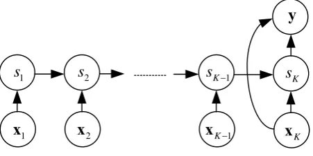
[image:2.595.49.275.273.386.2]s
−Fig. 1. Graphical model for IOHMM in the sequential variables
III. IOHMMMODEL
When IOHMM is applied to the batch system, the method for modeling sequential data is the chain structure that captures interactions between a sequence of inputs,
{
1, 2, , K}
=x x x " x , and the output vector, y. Thus, the number of sampling units in process variable trajectory measurements (x) is K; only one sampling point at the end of the batch is for quality measurements (y). IOHMM is trained to fit the conditional distribution probability P(y x)
of the output y given the input sequence x. The system structure is illustrated in Fig. 1. There is a set of hidden variables, s=
{
s1,",sK}
, and a fixed number of possible number of states. The conditional probability P(y x) can be written as a sum of term P( ,y sx) over all the possible state sequences,1 1
( ) ( , )
( , ) ( , )
s K
K K k k k
k s
P P s
P s P s s −
=
=
= Π
∑
∑
y x y x
y x x
(1)
Here the transition distribution parameterized by the softmax function [8]
{
1 2}
1 1 2
( k k , k) exp Tj j k
P s = j s − = j x ∝ λ ⋅x (2)
The emission (observation) distribution is characterized by a mixture of conditional linear Gaussians [9]
1
( , ) ( , )
M
K K m m
m
P s j N
=
= ∝ Π
y x μ Σ
(3) where the means (μm) of the distribution is time-variant and dependent on the input variables (xK),
0 T
m = m+ m K
μ μ b x . μ0m
is the vector determining the basis center of the Gaussian function and Σm is the covariance matrix. Thus, the parameters of the emission distribution,
{
0}
m = m m m
θ μ b Σ .
The parameter estimation of IOHMM can be approached by the maximum likelihood estimation. First, I sets of input-output sequences samples are collected,
(
)
{
}
{
, ; 1 ; 1, ,}
i i i i i
K
D= x y x = x " x i= " I ; then the set of all the parameters of the model
{
m,m 1, ,M; j j1 2, ,j j1 2 1, ,M}
Θ = θ = " λ = " is estimated.
The process of optimizing the parameters is iterative and it may take some time to converge. For a detailed description of the IOHMM learning algorithm, see [7].
IV. MPLS-BASED IOHMM FOR BATCH MONITORING
Although the IOHMM model approach performs a lot in different fields, it still has problems in the case of correlation inputs or limited data. In this paper, the integration of MPLS regression and IOHMM is proposed to formulate the probability model that can handle correlated inputs and limited observations. MPLS is applied to decomposing the variables into the lower dimensional ones in the orthonormal space. Then IOHMM is used to obtain information about the variability among batches for batch monitoring.
A. MPLS
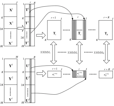
In the batch operation, when there are more than one process variable (J>1) and quality variable (M>1), a set of I number of historical batch data over K time intervals can be constructed into a three-way array and a two-way array shown in Fig. 2. The two-way data matrix, Y(I×M), is defined. The three-way data matrix is X(I× ×J K). Before performing MPLS, the data matrix X(I× ×J K) is unfolded to the two-dimensional matrix (I×KJ) (XStructure I of Fig. 2). Then each row of the data matrix for all process variables at one batch is rearranged to form a two-dimensional matrix with time×variables i( )
K×J
X . Each block matrix
( )
i
K×J
X is arranged from the top to the bottom, starting with the block corresponding to the first batch run. The resulting two-dimensional matrix has dimensions X(IK×J) (XStructure II of Fig. 2). Likewise, the quality variable is scaled in the same manner (Y Structure I of Fig. 2). In order to implement MPLS computation, the quality variables of each batch run are duplicated by K times to form
(IK×M)
to relate a set of predictor variables (X(IK×J)) to a set of response variables (Y(IK×M)).
X
X
K
I J
J 2J KJ
I J 1 i= 2K IK X 2 i=
[image:3.595.57.301.100.240.2]i=I K M I Y J 2K IK K Y 1 y 2 y I y 1 X 2 X I X
Fig. 2. Two unfolding structures for MPCA
Standard linear PLS can be viewed as a 2-stage process. Initially, an outer model is used to decompose X and Y blocks into scores (t ur, r) and loadings (p qr, r) based on the projection: 1 1 R T T r r r R T T r r r = = = + = + = + = +
∑
∑
X t p E TP E
Y u q F UQ F
(4)
where E and F are the residuals of X and Y, and R is the number of components used. The purpose of this step is to eliminate the interactions between process variables in the latent space. To find fitting regression for scores, an IOHMM probability model is developed and applied to the inner relation, i.e. ur =IOHMMr
( )
tr .B. MPLS-Based IOHMM Learning Algorithm
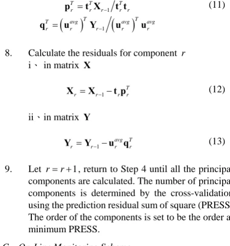
MPLS based IOHMM (IOHMM-MPLS) is a projection-based probability method that can be estimated in a sequential, stepwise manner. IOHMM-MPLS is different from the direct IOHMM modeling approach because the data are not used directly to train the IOHMM model. It is preprocessed by the PLS outer transform. The PLS outer projection is used as a dimensional reduction tool to remove collinearity. This will simplify the IOHMM model. Now the input variables are transformed to feature space variables, and then the probability model for transformed sequential data set is constructed.
In the decomposition procedures shown in Fig. 3, each component in the batch matrix Ti
is extracted over all the batches to form a component matrix Tr(K×I),
1 2
, 1, 2, ,
I
r =⎡⎣ r r r⎤⎦ r= R
T t t " t " (5)
Likewise, i( )
K×R
U represents the output scores
corresponding to each batch run. However, the final qualities at the end of each batch run should not depend upon the
separative Ui(K×R) at each time point; they should be settled together by the overall process operation scores with the single score. Thus, the average score ,
(1 ) avg i
R
×
u ,
revealing the pivotal information at the end of the batch run can be utilized as the modeling output steadily obtained by simply averaging all i( )
K×R
U within the batch run i.
, , ,
1 ,1 ,
1 1
1 K K
i avg i avg i avg i i
R k k R
k k
u u u u
K = =
⎡ ⎤
⎡ ⎤
=⎣ ⎦= ⎢ ⎥
⎣
∑
∑
⎦u " " (6)
Substituting , ,
, ,
1
( ) m
R
m sp m sp m T PLS i i r r
r u
=
=
∑
x q and , ,
1
( ) m
R
m m m T
PLS i i r r r u = =
∑
x q into (6),(
)
,1 ,2 ,
2 , , , 1 1 2 1
min ( )
2
min min min
m c i
m m m m
i i i Rm
R
m m sp m m T
i r i r r r
m m m
R
t t t
J u u
J J J
= ≅ − ⎡ ⎤ = ⎢ + + + ⎥ ⎣ ⎦
∑
x q "" (7)The pair of the score vectors (uri avg, and i r
t ) is used to build up the inner IOHMM probability model ( i avg, i, )
r r
P u t θ . The parameters of P u( ri avg, tir, )θ should be selected to maximize the likelihood probability estimation. The same training procedures in Section III can be directly applied. Consequently, as shown in Fig. 3, the distribution of the IOHMM model for each component, ( avg , )
r r
P u t θ ,
1, 2, ,
r= " R is trained.
1 J K K 2 IK 1 X 1 R K K 2 IK 2 X I X 2 T I T 1 T I K R T I K IOHMM1 1 M K K 2 IK 1 Y 1 R K K 2 IK 1 T 1 U 1 =
r r=R
r T I K r r I I 1 =
r r I r=R
2 Y I Y 2 U I U , 1 i avg u , i avg r
u i avg,
R
u
[image:3.595.307.547.463.686.2]IOHMMr IOHMMR
X
Y
IOHMM1 1
w
1
c
1
T
p
1
i
t
, 1
i avg
u c11
T
q
1
t
1
u
IOHMMr 2
w
2
c
2
T
p
2
i
t
, 2
i avg
u c12
T
q
2
t
2
u
IOHMMR
R
w
R
c
T R
p
i R
t
,
i avg R
u c1
T R
q
R
t
R
u
+ −
+ −
+ −
+ −
+ −
+ −
E
F
First Component Second Component Last Component
1, , i="I
1, ,
i="I i=1,",I 1, ,
i="I i=1,",I
[image:4.595.50.291.51.154.2]1, , i="I
Fig. 4. Sequential method of IOHMM-MPLS modeling: The data are
projected onto the latent scores, and then IOHMMs based on the scores
[image:4.595.310.545.52.303.2]are built up.
Fig. 4 shows the structure of the IOHMM-MPLS method. It uses the MPLS outer transform to generate sequential scores from the sequential data. The proposed IOHMM-MPLS algorithm can be formulated as follows:
1. Collect the historical batch data sets X(I× ×J K)
and Y(I×M) indicative of normal operations. The data should cover the range of the batch operating patterns and the conditions that yield accepted product quality.
2. Unfold data (X(I× ×J K)) batch-wiseX(I×KJ). Pre-treat X(I×KJ) and Y(I×M) using the mean and the standard deviation of each variable at each time in the batch cycle for all batches.
3. Rearrange the scaled X(I×KJ) and Y(I×M) into
(IK×J)
X and Y(IK×M). Let X0 =X(IK×J), 0 = (IK×M)
Y Y and r=1
4. For each r, take ur from one of columns of Yr−1
5. PLS outer transform i、in matrix X
1
T T T
r = r r− r r
w u X u u and normalize wr to norm 1 (8)
1
T
r = r− r
t X w
ii、in matrix Y
1
T T T
r = r r− r r
c t Y t t and normalize cr to norm 1 (9)
1
T
r = r− r u Y c
Keep doing this step iteratively until it converges. 6. Find the inner IOHMM probability model to get
maximum probability of the output score given a sequence of input scores
,
1
max log ( , )
I
i avg i r r i
P u
=
∑
t θ (10)The parameter estimation of IOHMM can be successfully solved by mean of the iterative EM algorithm.
7. Calculate X and Y loadings
1
T T T
r = r r− r r
p t X t t (11)
( )
1( )
T T
T avg avg avg
r = r r− r r
q u Y u u
8. Calculate the residuals for component r
i、in matrix X
1
T r = r− − r r
X X t p (12)
ii、in matrix Y
1
avg T r = r− − r r
Y Y u q (13)
9. Let r= +r 1, return to Step 4 until all the principal components are calculated. The number of principal components is determined by the cross-validation using the prediction residual sum of square (PRESS). The order of the components is set to be the order at minimum PRESS.
C. On-Line Monitoring Scheme
After modeling of IOHMM-MPLS, the model becomes
N N
explained unexplained
T
= +
X TP Ε (14)
N N
unexplained explained
T
= +
Y UQ F
For on-line monitoring of the measurement variables, the control limits should be built up at each sampling time point. As the new batch revolves, only the process values from the beginning of the batch till the current time (k) are available (X(k×J)). In order to fulfill the incomplete data set for on-line monitoring from the current time to the end of the batch, filling the missing values with the normal profile is applied here. Likewise, the output (yk(M×1)) is filled with the normal values. The score matrix by projecting the input and output data, (Xk(K×J) and yk(M×1)), mentioned above onto the loading matrices ( P and Q ) can be computed:
,1 ,2 ,
k =⎡⎣ k k k R⎤⎦= k
T t t " t X P (15)
,1 ,2 ,
k =⎡⎣ k k k R⎤⎦= k
U u u " u Y Q
The reconstructed score matrix and the corresponding unexplained matrix at each time point can be gotten by applying the trained IOHMM-MPLS,
,1 ,2 ,
k = ⎣⎡ k k k R⎤⎦
T t t " t (16)
,1 ,2 ,
( ,:) ( ,:)
k k k k J
T
k k
e e e k k
⎡ ⎤
= ⎣ ⎦
= −
e
X T P
"
(17)
, ,
( avg )
k r k r
P u t , r=1, 2,",R (18)
With the developed probability distribution that reflects the normal operation, control limits for the scores are required to detect any departure of the process from its standard behavior.
{ }, , ,
( ) 0.95
r r
avg
k r k r r r u
P u d du
Ω∈
=
∫∫
t
t t , 1, 2,r= ",R, (19)
Given the IOHMM model, the calculation results of the likelihood of these data are sorted. The data corresponding to 95% of the confidence level is taken to get the confidence bounds.
The squared prediction error ( Q kx( ) ) is statistically defined as
2
( )
x k
Q k = e (20)
The confidence limits of Q kx( ) cannot be determined directly from a particular distribution. The kernel density estimation [8] is used to determine the confidence limits.
V. ILLUSTRATION EXAMPLE
Data from a fed-batch penicillin fermentation [10] are used here to demonstrate the performance of the proposed method. The duration of each batch is 400hrs, comprising a pre-culture stage of about 45hrs and a fed-batch stage of about 355hrs. The sampling interval is 46.8 minutes. In the normal operating condition, small variations are added to the simulation input data to mimic process variation under the normal operating condition. Also, measurement noise is added to each of the monitoring variables. A total of 11 process variables are collected in each batch and a total of 50 batches based on the normal operation are used for the basis analysis. The quality variable is only measured at the end of the process. The simulation condition and the relevant parameters are the same as those of [10].
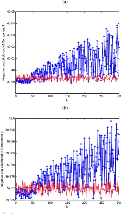
In the original problem, there are three types of abnormal conditions. Here only one of the fault conditions, which is the substrate feed rate linearly decreased from 0.042 to 0.032 and from the 40th hour till the end of the batch, is used for testing. A comparison between three different models, MPLS, IOHMM and IOHMM-MPLS, is made. For the abnormal batch, as shown in Fig. 5, the Qx or
2
T monitoring charts of MPLS do not detect this fault until the 100th hour of the batch run. Applying IOHMM to the same test batch, the results evidently shows that the control point has increased remarkably and fallen outside of the likelihood-based confidence limit after 75 hours of the batch run. (Due to the space limitation, the plot is not shown here.) The detection of process faults has been significantly improved after the sequential data is considered. For comparison, the control charts of IOHMM-MPLS are shown in Fig. 6. It can be seen that the proposed model can also detect the abnormal condition of this system earlier than MPLS. Moreover, the number of parameters in IOHMM-MPLS is 42, which is
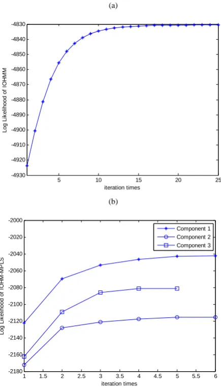
significantly less than in IOHMM which is 276. The smaller the number of parameters fitted, the lesser risk of overfitting the training data and therefore the lesser the occurrences of false alarms detected. Fig. 7 shows the comparison made between IOHMM and IOHMM-MPLS in terms of the EM training result of the two model likelihoods with respect to the iteration number for the training set. The proposed model enables the model training to converge faster and have higher probabilities. Thus, the proposed IOHMM-MPLS has the ability of capturing the actual process relationship between the variables under the noise environment.
0 50 100 150 200 250 300
0 10 20 30
T
2
0 50 100 150 200 250 300
0 10 20 30
[image:5.595.322.538.204.368.2]Qx
Fig. 5. Control charts for on-line monitoring in Example using MPLS. Each chart contains 95% (solid lines) of the control limit. The solid line with star signs represents the abnormal batch.
(a)
0 50 100 150 200 250 300
39.99 40 40.01 40.02 40.03 40.04 40.05
k
N
e
gat
iv
e L
og L
ik
e
lih
ood
of
C
om
p
one
nt
1
(b)
0 50 100 150 200 250 300
59.565 59.57 59.575 59.58 59.585 59.59 59.595 59.6
k
N
e
gat
iv
e Log
Li
k
el
ihoo
d of
C
om
p
onent
2
[image:5.595.321.527.421.784.2](c)
0 50 100 150 200 250 300
70.73 70.735 70.74 70.745 70.75 70.755 70.76 70.765 70.77 70.775
k
N
e
gat
iv
e L
og L
ik
e
lih
ood
of
C
om
p
one
nt
3
(d)
0 50 100 150 200 250 300
0 5 10 15 20 25 30 35 40 45
k
Qx
Fig. 6. (Con’t) Control charts for on-line monitoring in Example using IOHMM-MPLS: (a)-(c) IOHMM control chart of each score and (d) Qx
chart. Each chart contains 95% (solid lines) of the control limit. The solid line with star signs represents the abnormal batch.
VI. CONCLUSION
In view of on-line monitoring methods, the input and the output variables are first projected down onto a subspace of orthogonal latent variables to give the input and output scores. Then each pair of the latent variables is trained to build up the corresponding IOHMM probability density function. Unlike T2 control limits with the assumption of Gaussian distribution, the probability control limit for each component is sequentially calculated based on IOHMM probability density estimation and the bootstrap algorithm. Also unlike Qx control limits, the Kernel density function is used to construct the residue control limit. In comparison with conventional MPLS model, the proposed IOHMM-MPLS model shows negligible erroneous judgment on the normal operation condition and efficient monitoring capability to detect the time of occurrence of the process fault. Our extension work in the future will focus on the use of the IOHMM-MPLS model’s prediction on the diagnosis of fault patterns, and the application to the problem of multi-stage process systems instead of the single batch unit only.
(a)
5 10 15 20 25
-4930 -4920 -4910 -4900 -4890 -4880 -4870 -4860 -4850 -4840 -4830
iteration times
Log L
ik
el
iho
od of
I
O
H
M
M
(b)
1 1.5 2 2.5 3 3.5 4 4.5 5 5.5 6
-2180 -2160 -2140 -2120 -2100 -2080 -2060 -2040 -2020 -2000
iteration times
Lo
g Li
k
el
ih
ood
of
I
O
H
M
-M
P
L
S
Component 1 Component 2 Component 3
Fig. 7. (a) IOHMM and (b) IOHMM-MPLS model likelihoods concerning the EM iteratiive number in Example, in which three IOHMM-MPLS probability models are used for each input-output score.
REFERENCES
[1] P. Nomikos and J. F. MacGregor, “Multivariate SPC charts for monitoring batch processes,” Technometrics, 37, pp.41-59, 1995 [2] J. Chen and K.-C.Liu, “On-line batch process monitoring using
dynamic PCA and dynamic PLS models,” Chem. Eng. Sci., 57, pp.63-75, 2002.
[3] B. Lennox, G. A. Montague, H. G. Hiden, G. Kornfeld, P. Goulding, R., “Process monitoring of an industrial fed-batch fermentation,”
Biotechnol. Bioeng., 74, pp.125-138, 2001.
[4] S. J. Qin, “Statistical process monitoring: basics and beyond,” J.
Chemometrics, 17, pp.480-502, 2003.
[5] A. Cinar, S. J. Parulekar, C. Undey, G. Birol, Batch Fermentation:
Modeling, Monitoring and Control, Marcel Dekker, New York, NY,
2003.
[6] L. Rabiner, “A tutorial on hidden Markov models and selected applications in speech recognition,” Proc. IEEE, 76 (2) pp.257-286, 1989.
[7] Y. Bengio and P. Frasconi, “Input/output HMM’s for sequence processing,” IEEE Trans Neural Network, 3, pp.1231-1249, 1996. [8] C. M. Bishop, Neural Networks for Pattern Recognition, London, U.K.:
Oxford Univ. Press, 1995
[9] Y. Bengio, V.-P. Lauzon, and R. Ducharme, “Experiments on the application of IOHMMs to model financial returns series,” IEEE Trans
Neural Network, 12, pp.113-123,2001.
[image:6.595.63.274.61.427.2] [image:6.595.320.538.69.451.2]