Proceedings of NAACL-HLT 2019, pages 1968–1976 1968
Generating Knowledge Graph Paths from Textual Definitions
using Sequence-to-Sequence Models
Victor Prokhorov,1Mohammad Taher Pilehvar1,2 and Nigel Collier1 1Department of Theoretical and Applied Linguistics, University of Cambridge 2School of Computer Engineering, Iran University of Science and Technology, Tehran, Iran
[email protected], [email protected], [email protected]
Abstract
We present a novel method for mapping un-restricted text to knowledge graph entities by framing the task as a sequence-to-sequence problem. Specifically, given the encoded state of an input text, our decoder directly predicts paths in the knowledge graph, starting from the root and ending at the target node fol-lowing hypernym-hyponym relationships. In this way, and in contrast to other text-to-entity mapping systems, our model outputs hierar-chically structured predictions that are fully in-terpretable in the context of the underlying on-tology, in an end-to-end manner. We present a proof-of-concept experiment with encourag-ing results, comparable to those of state-of-the-art systems.
1 Introduction
Text-to-entity mapping is the task of associating a text with a concept in a knowledge graph (KG) or an ontology (we use two terms, interchange-ably). Recent works (Kartsaklis et al.,2018;Hill
et al.,2015) use neural networks to project a text
to a vector space where the entities of a KG are represented as continuous vectors. Despite being successful, these models have two main disadvan-tages. First, they rely on a predefined vector space which is used as a gold standard representation for the entities in a KG. Therefore, the quality of these algorithms depends on how well the vector space is represented. Second, these algorithms are not interpretable; hence, it is impossible to understand why a certain text was linked to a particular entity. To address these issues we propose a novel tech-nique which first represents an ontology concept as a sequence of its ancestors in the ontology (hy-pernyms) and then maps the corresponding textual description to this unique representation. For ex-ample, given the textual description of the concept swift(“small bird that resembles a swallow and is
noted for its rapid flight”), we map it to the hier-archical sequence of entities in a lexical ontology: animal→chordate→vertebrate→bird→ apod-iform bird. This sequence of nodes constitutes a path.1
Our model is based on a sequence-to-sequence neural network (Sutskever et al., 2014) coupled with an attention mechanism (Bahdanau et al., 2014). Specifically, we use an LSTM (
Hochre-iter and Schmidhuber, 1997) encoder to project
the textual description into a vector space and an LSTM decoder to predict the sequence of entities that are relevant to this definition. With this frame-work we do not need to rely on the pre-existing vector space of the entities, since the decoder ex-plicitly learns topological dependencies between the entities of the ontology. Furthermore, the pro-posed model is more interpretable for two rea-sons. First, instead of the closest points in a vector space, it outputs paths; therefore, we can trace all predictions the model makes. Second, the atten-tion mechanism allows to visualise which words in a textual description the model selects while pre-dicting a specific concept in the path. In this paper, we consider rooted tree graphs2only and leave the extension of the algorithm for more generic graphs to future work.
We evaluate the ability of our model in generat-ing graph paths for previously unseen textual def-initions on seven ontologies (Section3). We show that our technique either outperforms or performs on a par with a competitive multi-sense LSTM model (Kartsaklis et al., 2018) by better utilising external information in the form of word embed-dings. The code and resources for the paper can
1We only consider hypernymy relations, from the root to
the parent node (apodiform bird) of the entityswift.
2Only single root is allowed. If a tree has more than one
be found at https://github.com/VictorProkhorov/
Text2Path.
2 Methodology
We assume that an ontology is represented as a rooted tree graph G = (V, E, T), where V is a set of entities (e.g. synsets in WordNet), E is a set of hyponymy edges, andT is a set of textual descriptions such that∀v∈V there is atv ∈T.
2.1 Node representation
We assume that an ontological concept can be de-fined by either using a textual description from a dictionary or hypernyms of the defining concept in the ontology. For example, to define the nounswift one can use the dictionary definition mentioned previously. Alternatively, the concept ofswiftcan be understood from its hypernyms, e.g. in the triv-ial case one can say thatswiftis an animal. This definition is not very useful sinceanimalis a hy-pernym for many other nouns. To provide a more specific definition, one can use a sequence of hy-pernyms e.g.animal→chordate→vertebrate→
bird→apodiform birdstarting from the most ab-stract node (root of an ontology) to the most specif (parent node of the noun).
More formally, for each entity v 6= vroot ∈ V we create a pathpv. Eachpv starts fromvrootand ends with a hypernym of v, i.e., the hierarchical order of entities is preserved. Then the pathpv is aligned withtv such that each node is defined by a textual definition and a path. This set of aligned representations is used to train the model.
The path representation of an entity ends with its parent node. Therefore, a leaf node will not be present in any of the paths. This is problematic if a novel definition should be attached to a leaf. To alleviate this issue we employ the “dummy source sentences” technique from neural machine trans-lation (NMT) (Sennrich et al., 2016). We create an additional set of paths from the root node to each leaf. As for the textual definition we leave it empty.
2.2 Model
We use a sequence-to-sequence model with an at-tention mechanism to map a textual description of a node to its path representation.
Encoder. To encode a textual definition tv = (wi)Ni=1, whereN is sentence length, we first map each wordwi to a dense embeddingewi and then
use a bi-directional LSTM to project the sequence into a latent representation. The final encoding state is obtained by concatenating the forward and backward hidden states of the bi-LSTM.
Decoder. Decoding the path representation of a node from the latent state of the textual descrip-tion is done again with an LSTM decoder. Sim-ilarly to the encoding stage, we map each sym-bol in the path pv = (sj)Mj=1 to a dense em-bedding esj, where M is the path length. To
calculate the probability of the path symbol sj at time step j we first represent the path se-quence as h∗j = LSTM(esj, h∗j−1). Then, we concatenate h∗j with the context vector cj (de-fined next) and pass the concatenated repre-sentation [h∗j;cj] through the softmax function, i.e. sj = max(softmax(W[h∗j;cj])), where
W is a weight parameter. To calculate the
context vector cj we use an attention mecha-nism, eji = vTatanh(Wahi +Uah∗j) and cj = PN
i softmax(eji)hi, where va, Wa and Ua are
the weight parameters, over the words in the text description.
3 Experimental Setup
Ontologies. We experimented with seven graphs four of which are related to the bio-medical do-main: Phenotype And Trait Ontology3 (PATO), Human Disease Ontology (Schriml et al., 2012,
HDO), Human Phenotype Ontology (Robinson
et al., 2008, HPO) and Gene Ontology4 (
Ash-burner et al.,2000, GO). The other three graphs,
i.e. WNanimal.n.015, WNplant.n.02 and WNentity.n.01 are subgraphs of the WordNet 3.0 (Fellbaum, 1998). We present the statistics of the graphs in Table1.
Ontology Preprocessing. All the ontologies we experimented with are represented as directed acyclic graphs (DAGs). This creates an ambiguity for node path definitions since there are multiple pathways from a root concept to other concepts. We have assumed that a single unambiguous path-way will reduce the complexity of the problem and leave the comparison with ambiguous pathways (which would inevitably involve a more complex model) to future work. To convert a DAG to a tree
3
http://www.obofoundry.org
4
After prerocessing GO we took its largest connected component.
5The subscript in ‘WN’ indicates the name of the root
Graphs |V| Depth Branch A.D
PATO 1742 (4.94,10) (3.95,92) 20 WNanimal.n.01 3999 (6.94,12) (3.79,52) 26
WNplant.n.02 4487 (4.70,9) (5.91,357) 28
HDO 9095 (5.92,12) (4.59,222) 27 HPO 13348 (6.95,14) (3.40,32) 24 GO 29682 (6.40,14) (3.28,172) 21 WNentity.n.01 74374 (8.01,18) (4.52,402) 36
Table 1: Statistics of the Graphs.|V|is the number of nodes,depthis the path length from the root of a graph to a node,branchis the number of neighbours a node has (leaves were removed from the calculation). The first value in the parentheses corresponds to the average and the second to the maximum value. A.D stands for average number of decisions the model makes to infer a path, i.e A.D = average depth×average branch.
we constrain each entity to have only one parent node. The edges between the other parent nodes are removed.6
Path Representations. We also experiment with two path representations. Our first approach, text2nodes, uses the label of an entity (cf. Section 1) to represent a path. This is not efficient since the decoder of the model needs to select between all of the entities in an ontology and also requires more parameters in the model. Our second approach, text2edges, to reduce the number of symbols for the model to choose from, uses edges to represent the path. To do this we create an artificial vocabu-lary of the size∆(G), where∆(G)corresponds to the maximum degree of a node. Each edge in the graph is labeled using the artificial vocabulary. For the example in Section 1, the path would be an-imal −[a]→ chordate −[b]→ vertebrate −[c]→
bird−[d]→apodiform birdwhere{a,b,c,d}is the artificial vocabulary. In the resulting path we dis-card labels for the entities; therefore, the path re-duces to: [a]→[b]→[c]→[d].
3.1 Baselines
Bag-of-Words Linear Regression (BOW-LR):
To represent a textual definition in a vector space we first use a pre-trained set of word embeddings
(Speer et al.,2017) to represent words in the
def-inition and then find the mean of the word em-beddings. As for the ontology, we use node2vec
(Grover and Leskovec, 2016), to represent each
entity in a vector space. To align the two vector spaces we use linear regression.
6The choice of an edge is performed on random basis.
Multi-Sense LSTM (MS-LSTM): Kartsaklis
et al.(2018) proposed a model that achieves
state-of-the-art results on the text-to-entity mapping on the Snomed CT7 dataset. The approach uses a novel multi-sense LSTM, augmented with an at-tention mechanism, to project the definition to the ontology vector space. Additionally, for a better alignment between the two vector spaces, the au-thors augmented the ontology graph with textual features.
3.2 Evaluation Metric
To perform evaluation of the models described above we used Ancestor-F1 score (Mao et al., 2018). This metric compares the ancestors (is−
amodel) of the predicted node with the ancestors (is−agold) of the gold node in the taxonomy.
P = |is−amodel∧is−agold|
|is−amodel| ,
R= |is−amodel∧is−agold|
|is−agold|
,
where P and R are precision and recall, respec-tively. The Ancestor-F1 is then defined as:
2×P×R
P+R.
3.3 Intrinsic Evaluation
To verify the reliability of our model on text-to-entity mapping we did a set of experiments on the seven graphs (Section3) where we map a textual definition of a concept to a path.
To conduct the experiments we randomly sam-pled 10% of leaves from the graph. From this sample, 90% are used to evaluate the model and 10% are used to tune the model. The remaining nodes in the graph are used for training. We sam-ple leaves for two reasons: (1) to predict a leaf, the model needs to make the maximum number of (correct) predictions and (2) this way we do not change the original topology of the graph. Note that the sampled nodes and their textual definitions are not present in the training data.
Both baselines predict a single entity instead of a path. To have the same evaluation framework for all the models, for each node predicted by the baselines we create8 a path from the root of the node to the predicted node. However, we want
7
https://www.snomed.org/snomed-ct
8We used NetworkX (https://networkx.github.io) to find a
Models PATO WNanimal.n.01 WNplant.n.02 HDO HPO GO WNentity.n.01
BOW-LR 0.79 0.75 0.65 0.55 0.63 0.32 0.41 MS-LSTMλ= 0 0.77 0.73 0.62 0.70 0.72 0.69 0.51
MS-LSTMλ= 0.5 0.80 0.76 0.65 0.70 0.73 0.70 0.57
MS-LSTMλ= 1 0.75 0.66 0.57 0.65 0.63 0.62 0.51
[image:4.595.84.517.63.187.2]text2nodes 0.75 0.66 0.66 0.69 0.62 0.67 0.60 text2edges 0.76 0.68 0.66 0.69 0.69 0.69 0.61 MS-LSTM∗λ=0.5 0.81 0.76 0.66 0.71 0.74 0.71 0.58 text2nodes∗ 0.83 0.71 0.68 0.71 0.69 0.70 0.62 text2edges∗ 0.83 0.77 0.70 0.73 0.74 0.72 0.65
Table 2: Ancestor F1 results. Numbers in bold represent the best performing system on a graph. Models marked with∗ make use of pre-trained word embedding in their encoder. Lambda (λ) is defined in Section3.1. We use the same number of epochs, batch size and number of latent dimensions both for MS-LSTM and our models (AppendixC).
to emphasize that this is disadvantageous for our model, since all the symbols in the path are pre-dicted by it and in the case of the baselines only a single node is predicted.
The results are presented in Table 2. Mod-els that are in the last three rows of Table 2 use pre-trained word embeddings (Speer et al.,
2017) in the encoder. MS-LSTM and our
mod-els that are above the last three rows use ran-domly initialised word vectors. We had four ob-servations: (1) without pre-trained word embed-dings in the encoder our model outperforms the best MS-LSTMλ= 0.5 only on two of the seven graphs, (2) the text2edges∗model outperforms all the other models including MS-LSTM∗λ=0.5, (3) the text2edges model can better exploit pre-trained word embeddings than MS-LSTM, (4) our model performs better when the paths are represented us-ing edges (rather than nodes). We also found that there is a strong negative correlation (Spearman:
−0.75, Pearson: −0.80) between A.D. (Table 3) and the Ancestor F1 score for the text2edges∗ model, meaning that with an increase in A.D. the Ancestor F1 score decreases.
3.4 Error Analysis
We carried out an analysis on the outputs of our best-performing model, i.e. text2edges∗ with pre-trained word embeddings. One factor that affects the performance is the number of in-valid sequences predicted by the text2nodes and text2edges models. An invalid sequence is the path that does not exist in the original graph. This happens because at each time step the decoder out-puts a distribution over all the nodes/edges and not just over possible children nodes. We
there-fore performed a count of the number of invalid sequences produced by the model. The percentage of invalid sequences is in the range of 1.82% -8.50% (AppendixB), which is relatively low. This analysis was also performed by J. Kusner et al. (2017). To guarantee that the model always pro-duces valid graphs, they use a context-free gram-mar. A similar method can be adapted in our work.
0 1 2 3 4 5 6 7 8 9 10
Length of Sequence
0 100 200 300 400 500 600 700 800
Frequency
PATO graph
2 3 4 5 6 7 8
Gold Sequence Length
2 3 4 5 6 7 8
Decoded Sequence Length
PATO graph gold performance
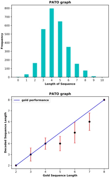
[image:4.595.312.502.394.702.2]Another factor that affects the performance is the length of the generated paths which is expected to match the length of the gold path. To test this, we compared the mean length of the generated se-quences with the length of the gold path (the graph on the bottom of Figure 1). Also, in the training set, we associate the length of the sequences with their frequencies (the graph on the top of Figure 1). We found that (1) the length of the generated paths are biased towards the more frequent paths in the training data, (2) if the length of a path is not frequent in the training data, the model either under-generates or over-generates the length (Ap-pendixD).
4 Related Work
Text-to-entity mapping is an essential component of many NLP tasks, e.g. fact verification (Thorne
et al., 2018) or question answering (Yih et al.,
2015). Previous work has approached this prob-lem with pairwise learning-to-rank method (
Lea-man et al.,2013) or phrase-based machine
transla-tion (Limsopatham and Collier, 2015). However, these methods generally ignore ontology’s struc-ture. More recent work has viewed the problem of text-to-entity mapping as a projection of a tex-tual definition to a single point in a KG (
Kartsak-lis et al., 2018; Hill et al., 2015). However,
de-spite potential advantages, such as being more in-terpretable and less brittle (model predicts multi-ple related entities instead of one), path-based ap-proaches have received relatively little attention. Instead of predicting a single entity, path-based models, such as the one we proposed in this paper, try to map a textual definition to multiple relevant entities in an external resource.
5 Conclusion and Future Work
We presented a model that maps textual defini-tions to interpretable ontological pathways. We evaluated the proposed technique on seven seman-tic graphs, showing that it can perform competi-tively with respect to existing state-of-the-art text-to-entity systems, while being more interpretable and self-contained. We hope this work will en-courage further research on path-based text-to-entity mapping algorithms. A natural next step will be to extend our framework to DAGs. Fur-thermore, we plan to constrain our model to al-ways predict paths that exist in the graph, as we discussed above.
Acknowledgments
We would like to thank the anonymous reviewers for their comments. Also, we would like to thank Dimitri Kartsaklis and Ehsan Shareghi for helpful discussions and comments. This research was sup-ported by an EPSRC Experienced Researcher Fel-lowship (N. Collier: EP/M005089/1) and an MRC grant (M.T. Pilehvar: MR/M025160/1). We grate-fully acknowledge the donation of a GPU from the NVIDIA Grant Program.
References
Michael Ashburner, Catherine A. Ball, Judith A. Blake, David Botstein, Heather Butler, J. Michael Cherry, Allan P. Davis, Kara Dolinski, Selina S. Dwight, Janan T. Eppig, Midori A. Harris, David P. Hill, Lau-rie Issel-Tarver, Andrew Kasarskis, Suzanna Lewis, John C. Matese, Joel E. Richardson, Martin Ring-wald, Gerald M. Rubin, and Gavin Sherlock. 2000.
Gene ontology: tool for the unification of biology.
Nature Genetics, 25(1):25–29.
Dzmitry Bahdanau, Kyunghyun Cho, and Yoshua Bengio. 2014. Neural machine translation by jointly learning to align and translate. CoRR, abs/1409.0473.
Christiane Fellbaum, editor. 1998. WordNet: An Elec-tronic Database. MIT Press, Cambridge, MA.
Aditya Grover and Jure Leskovec. 2016. node2vec: Scalable feature learning for networks. CoRR, abs/1607.00653.
Felix Hill, Kyunghyun Cho, Anna Korhonen, and Yoshua Bengio. 2015. Learning to understand phrases by embedding the dictionary. CoRR, abs/1504.00548.
Sepp Hochreiter and J¨urgen Schmidhuber. 1997. Long short-term memory. Neural Comput., 9(8):1735– 1780.
Matt J. Kusner, Brooks Paige, and Jos Miguel Hernndez-Lobato. 2017. Grammar variational au-toencoder.
Dimitri Kartsaklis, Mohammad Taher Pilehvar, and Nigel Collier. 2018. Mapping text to knowledge graph entities using multi-sense lstms. In Proceed-ings of the 2018 Conference on Empirical Methods in Natural Language Processing, pages 1959–1970. Association for Computational Linguistics.
Robert Leaman, Rezarta Dogan, and Zhiyong lu. 2013.
Nut Limsopatham and Nigel Collier. 2015. Adapt-ing phrase-based machine translation to normalise medical terms in social media messages. CoRR, abs/1508.02285.
Yuning Mao, Xiang Ren, Jiaming Shen, Xiaotao Gu, and Jiawei Han. 2018. End-to-end reinforcement learning for automatic taxonomy induction. In Pro-ceedings of the 56th Annual Meeting of the Associa-tion for ComputaAssocia-tional Linguistics (Volume 1: Long Papers), pages 2462–2472. Association for Compu-tational Linguistics.
Peter N. Robinson, Sebastian K¨ohler, Sebastian B Bauer, Dominik Seelow, Denise Horn, and Stefan Mundlos. 2008. The human phenotype ontology: a tool for annotating and analyzing human hereditary disease. American journal of human genetics, 83 5:610–5.
Lynn M. Schriml, Cesar Arze, Suvarna Nadendla, Yu-Wei Wayne Chang, Mark Mazaitis, Victor Felix, Gang Feng, and Warren A. Kibbe. 2012. Disease ontology: a backbone for disease semantic integra-tion. InNucleic Acids Research.
Rico Sennrich, Barry Haddow, and Alexandra Birch. 2016. Improving neural machine translation mod-els with monolingual data. In Proceedings of the 54th Annual Meeting of the Association for Compu-tational Linguistics (Volume 1: Long Papers), pages 86–96. Association for Computational Linguistics.
Robert Speer, Joshua Chin, and Catherine Havasi. 2017. Conceptnet 5.5: An open multilingual graph of general knowledge.
Ilya Sutskever, Oriol Vinyals, and Quoc V. Le. 2014.
Sequence to sequence learning with neural net-works.CoRR, abs/1409.3215.
James Thorne, Andreas Vlachos, Christos Christodoulopoulos, and Arpit Mittal. 2018.
Fever: a large-scale dataset for fact extraction and verification. In Proceedings of the 2018 Conference of the North American Chapter of the Association for Computational Linguistics: Human Language Technologies, Volume 1 (Long Papers), pages 809–819. Association for Computational Linguistics.
Wen-Tau Yih, Ming-Wei Chang, Xiaodong He, and Jianfeng Gao. 2015. Semantic parsing via staged query graph generation: Question answering with knowledge base. InACL.
A DAGs
Graphs Mult.P% AV.P
PATO 31.29 2.97
WNanimal.n.01 0.88 2.00
WNplant.n.02 0.16 2.00
HDO 16.23 2.13
HPO 23.24 2.23
GO 64.01 2.77
[image:6.595.316.515.86.203.2]WNentity.n.01 1.91 2.03
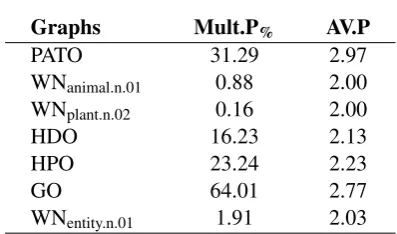
Table 3: Statistics of nodes with multiple inheritance. Mult.P%stands for percentage of nodes with more than
one parent node. AV.P stands for average number of parents a node with multiple inheritance has.
B Invalid Sequences
Graphs Invalid% Ntotal
PATO 1.82 110
WNanimal.n.01 4.56 263
WNplant.n.02 2.23 314
HDO 4.02 622
HPO 7.08 847
GO 6.94 1845
WNentity.n.01 8.50 5191
Table 4: Statistics of invalid sequences. Invalid%is the
percentage of invalid sequences and Ntotal is the total
number of sequences that were tested.
C Settings for Models
BOW-LR: To represent an ontology in a vector space we use node2vec https://snap.stanford.edu/
node2vec/. For all the graphs the following
hyper-parameters of the algorithm are the same: walk-length= 5,window-size=5anditer=40. As for the number of dimensions we set it to 128 for PATO,
WNanimal.n.01, WNplant.n.02, HDO and HPO graphs.
For GO and WNentity.n.01 graphs we set it to 256. All the other parameters of node2vec are default.
We do not modify the numberbatch
em-beddings https://github.com/commonsense/
conceptnet-numberbatch. If a word in a textual
definition is missing we initilised the embedding for this word with zeros.
[image:6.595.313.519.310.422.2]2 3 4 5 6 7 8 Gold Sequence Length
2 3 4 5 6 7 8
Decoded Sequence Length
PATO graph gold performance
0 1 2 3 4 5 6 7 8 9 10 Length of Sequence
0 100 200 300 400 500 600 700 800
Frequency
PATO graph
0 1 2 3 4 5 6 7 8 9 10 11 Gold Sequence Length
0 1 2 3 4 5 6 7 8 9 10
Decoded Sequence Length
WordNet Animal graph gold performance
0 1 2 3 4 5 6 7 8 9 10 11 12 Length of Sequence
0 200 400 600 800 1000
Frequency
WordNet Animal graph
0 1 2 3 4 5 6 7 8 Gold Sequence Length
2 3 4 5 6
Decoded Sequence Length
WordNet Plant graph gold performance
0 1 2 3 4 5 6 7 8 9 Length of Sequence
0 250 500 750 1000 1250 1500 1750 2000
Frequency
WordNet Plant graph
1 2 3 4 5 6 7 8 9 10 11 Gold Sequence Length
2 3 4 5 6 7 8
Decoded Sequence Length
HDO graph gold performance
0 1 2 3 4 5 6 7 8 9 10 11 Length of Sequence
0 500 1000 1500 2000 2500 3000 3500
Frequency
[image:7.595.104.481.62.660.2]HDO graph
2 3 4 5 6 7 8 9 10 11 12 13 Gold Sequence Length
3 4 5 6 7 8 9 10 11 12
Decoded Sequence Length
HPO graph gold performance
0 1 2 3 4 5 6 7 8 9 10 11 12 13 14 Length of Sequence
0 500 1000 1500 2000 2500 3000 3500 4000
Frequency
HPO graph
1 2 3 4 5 6 7 8 9 10 11 12 Gold Sequence Length
3 4 5 6 7 8 9 10
Decoded Sequence Length
GO graph gold performance
0 1 2 3 4 5 6 7 8 9 10 11 12 13 14 Length of Sequence
0 1000 2000 3000 4000 5000 6000 7000 8000
Frequency
GO graph
1 2 3 4 5 6 7 8 9 10 11 12 13 14 15 16 17 Gold Sequence Length
4 5 6 7 8 9 10 11 12 13 14 15 16
Decoded Sequence Length
WordNet Entity graph gold performance
0 1 2 3 4 5 6 7 8 9 10 11 12 13 14 15 16 17 18 Length of Sequence
0 5000 10000 15000 20000 25000
Frequency
[image:8.595.106.480.65.507.2]WordNet Entity graph
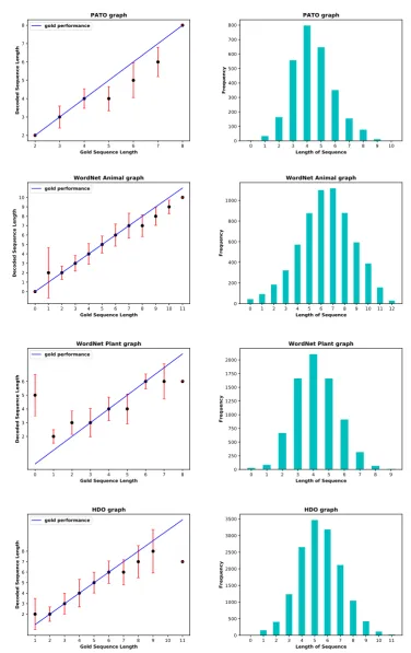
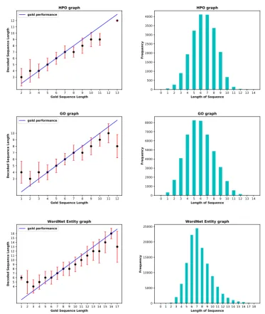
Figure 3: Continuation of Figure2. On the left graphs show: length of gold sequence vs mean length of decoded sequence on a test set; On the right graphs show: length of sequence vs length frequency on a training set.
MS-LSTM: There are only two hyper-parameters that we vary during the embedding of ontology concepts: λ(we report the values in the paper) and the embedding size of the con-cepts. We set it to 128 for PATO, WNanimal.n.01,
WNplant.n.02, HDO and HPO graphs. For GO and
WNentity.n.01graphs we set it to 256.
For all the graphs the model is trained for 300 epochs, dimensions of word embeddings is set to 64 and bi-LSTM is used instead of LSTM. Batch size is set to 16 and the number of latent dimen-sions in bi-LSTM is set to 128 for the PATO,
WNanimal.n.01, WNplant.n.02, HDO and HPO graphs.
For GO and WNentity.n.01 graphs we set these
pa-rameters to 128 and 256 respectively. All the other hyper-parameters are default.
When we use pre-trained word
em-beddings we reduce (with PCA https:
//scikit-learn.org/stable/modules/generated/
sklearn.decomposition.PCA.html) its dimensions
from 300 to 64.
Our Model: For all the graphs the model is trained for 300 epochs, dimensions of word embeddings (also for node/edges embeddings) is set to 64 and bi-LSTM is used in the encoder
and LSTM in the decoder. Batch size is set
128 for the PATO, WNanimal.n.01, WNplant.n.02, HDO and HPO graphs. For GO and WNentity.n.01 graphs we set these parameters to 128 and 256
respectively. For optimizer we used RMSProp
(https://www.tensorflow.org/api docs/python/tf/
train/RMSPropOptimizer) with learning rate =
0.001.
When we use pre-trained word
em-beddings we reduce (with PCA https:
//scikit-learn.org/stable/modules/generated/
sklearn.decomposition.PCA.html) its dimensions
from 300 to 64.
D Length of Generated Path