Abstract—An algorithm based on the Bayesian approach to detect and recognise off-axis pulse laser beams propagating in the atmosphere is presented. This method optimises the off-axis measurement of pulse laser with low energy level by ultra fast cameras.
The performance of this technique is validated with simulated signals obtained from array sensor.
Index Terms— Array, Bayesian, detection, laser, sensor.
INTRODUCTION
As lasers are coming into more and more widespread use in target-designation, countermeasures, range finding, and surveying operations, the potential for accidental damage to human eyes or sensors on the battlefield increases. Initial indications are off-axis laser beam detection shows promise for use as an early laser warning system.
The laser beams can indeed be off-axis detected when propagating in the lower atmosphere by their scattering track on natural aerosols [1]. In the last years, several laboratories have conducted studies to detect off-axis non cooperative pulsed laser beams in the lower atmosphere.
A problem of interest in laser imager processing occurs when Signal to Noise Ratio is very low. For instance, for a sub-optimum leading-edge level detection procedure, the noise may increased the probability false alarm (pfa) if the level is low.
To decrease the pfa a Bayesian approach is used in which a probability density function (pdf) for the signal amplitude is used as prior distribution in determining the pdf for signal plus noise [2].
This paper describes an analytic model of scattered light under different atmospheric and angle conditions in a 3D geometry, giving the photometry, the geometry and the temporal parameters of the detected signal.
Then, to evaluate the detection technique, a computer code is developed.
* T. Gaudo is with the “Office National Études et de Recherches Aérospatiales” O.N.E.R.A (The French Aerospace Lab), Palaiseau 91761 France (phone: +33-01-69-93-63-74; thierry.gaudo@ onera.fr).
Following this theoretical part, simulations in the visible and near infrared bands are presented with a kilometric scale of free laser propagation. The technique developed for this purpose confirms a pfa reduction that allows to improve Off-Axis Laser Warning detection.
In section 2, an analytic model describing the physics of the detection is presented. Section 3 is devoted to the simulations and detection analysis. Section 4 summarizes and concludes the discussion.
LASERDETECTIONMODELDESCRIPTION
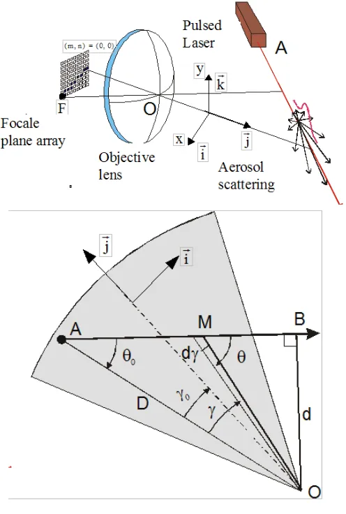
The objective of the model is to calculate the parameters of the light scattered by a pulsed beam onto atmosphere aerosols, in order to estimate the potential performances of a dedicated warning sensor. So, the power received on a 2D array of detectors is calculated, coming from the scattered beam, the geometric image of the beam on the focal plane array, and the time and duration of the pixel illumination. This energy is assumed to be detected by a 2D-array sensor.
Photometry in 3D geometry
Considering the laser beam and the sensor in a 3D geometry as in Fig. 1. O is the center of the detection optics. A is the source of the laser beam : D = OA. The orthogonal distance from O to the beam is : d = 0B. M is a point on the beam, observed with an angle γ from O, in respect with the source direction. θ is the angle between the observation axis and the beam . A is observed with an angle γ0 from 0. θ0 is the angle
between the observation axis and the beam. The laser beam is modeled as a thin line, i.e. the image of its right section is smaller than the pixel in the focal plane.
The atmospheric parameters depending on altitude h are : α(h) : absorption coefficient (m-1), assumed to be constant on the beam, β(h) : scattering coefficient (m-1), assumed to be constant on the beam. The scattering distribution is given by the phase function ϕ(θ,h) . Ac is the sensor collection area, Ee is the pulse energy.
Pe(t) is the time dependent transmitted power of the laser. Pe(t) is supposed having a gaussian shape with a 1/e2 width τ
e. Time origin t=0 is set at the center of the pulse.
2 A
e e 2
e e
2
2
t
P (t)
E
exp
8
τ
π
τ
π
τ
π
τ
π
ττττ
=
−
(1)
Optimal Recognition Algorithm for Cameras of
Lasers Evanescent
Figure 1 Detection geometry – 3D and plane view
The incident laser power at M is expressed as :
{
}
(
)
M A
i e
AM
P
(t)
P (t
) exp
AM
c
α β
α β
α β
α β
=
−
−
+
(2)The scattered power at M by a beam element of length dL in the direction
θθθθ
into a solid angled
Ω
is :M A
d i
dP
(t)
=
P (t)
βϕ
βϕ
βϕ
βϕ
Ω
dL
(3) Geometric considerations as in Fig. 1 give :AB ct
AM
AB j
=
(4)
MO
=
AO AM
−
(5)
h
=
OM k
(6)MO AB
arccos
MO AB
θθθθ
=
(7)
0
γ θ θ
γ θ θ
γ θ θ
γ θ θ
= −
(8)(
)
c 0
2
A cos
d
MO
γ
γ
γ
γ
γ
γ
γ
+
γ
Ω =
(9)
The cosine term comes from the field angle between the scattered beam and the optical axis.
( )
MO d
dL
c dt
sin
γγγγ
θθθθ
=
=
(10)
After propagation from M to O, the received power at the sensor aperture, coming from the beam in the direction θ into the angle element dγ is :
{
}
(
)
M A
r d
MO
dP
(t)
P (t
) exp
MO
c
α β
α β
α β
α β
=
−
−
+
(11) By replacing the expressions (2), (3), (4), (5), (6),(7), (8), (9), (10) into (11) the power received on O becomes :
(
)
{
}
(
)
(
)
O
c 0
A r
e 0 2
A cos
c
dP (t)
P (t
)
G(t)
dt
MO
G(t)
exp
AM
MO
+
=
−
=
−
+
+
γ
γ
γ
γ
γ
γ
γ
γ
τ βϕ
τ βϕ
τ βϕ
τ βϕ
α β
α β
α β
α β
(12)
with the arrival time on the lens :
0
AM
MO
c
ττττ
=
+
(13)
The optical parameters depends of the instrumental transmission factor τi, of the focal F, of the optic modulation response and of the array dimension.
Considering the detection plane parallels to the plane formed by the sensor input lens, the vector drawing the laser trace on the array is expressed as :
OF
=
F
(
)
{
}
(
)
(
)
F c 0 A ri e 0 2
A cos
c
dP (t)
P (t
)
G(t)
dt
MO
G(t)
exp
AM
MO
+
=
−
=
−
+
+
γ
γ
γ
γ
γ
γ
γ
γ
τ
τ βϕ
τ
τ βϕ
τ
τ βϕ
τ
τ βϕ
α β
α β
α β
α β
(15)
By considering the quasi-perfect objective, the optic modulation response is a spot of Airy. The geometrical form of this response can be approached by Sp a circular surface of angular rp radius limited by solid angle dΩ (9). Surface lit according to direction x and y in the array plane is:
p
p p
S (x, F, y) 1
x
y
d
if arctan
arctan
r
F
F
2
S (x, F, y)
0 elsewhere
−
=
Ω
+
< <
−
=
(
16)
With (16) laser trace drawn on the detection plane (15) becomes (* convolution operator) :
F
r r
p
dP (t)
dP (t)
*S
dt
=
dt
(17)Detection plane dimensions describes by a matrix 2D are of Nsit pixels in vertical direction Ngis pixels in horizontal direction. the pixels are of width lgis, length lgis. From these parameters the laser trace imaged by the array sensor is expressed by :
( )
r
l lsit gis ym xn
N 1
Nsit 1 gis 2 2
F
r n
m 0 n 0 lsit lgis ym xn
2 2
dP (t, m, n)
dt
dP (t)dxdy
F
+ + − − = = − −
=
∑ ∑
∫
∫
δδδδ
(18) its spatial sampling step if one considers the axis of the lens in the array center and the located pixel (m, n) = (0,0) placed as shown in the Fig. 1 is:
gis gis n n m sit sit
N
1
n
l
x
2
2
F
y
N
1
m
l
2
2
+ −
=
=
− −
(19)amplifies filters and samples each pixel. The deterministic signal at the output of filter modeled with the H(t) pulse response is assumed to take the form :
r
V(t, m, n)
=
H(t, m, n) * P (t, m, n)
(20)Electronic signal from each pixel line is processed in one channel data sampler working at Ts . The V signal provides the amplitude evolution of received power for different pixels in vertical and horizontal plane. This signal imaging laser spot on array sensor is written :
( )
s N 1 M 1(
s)
n 0 m 0
V kT
V kT , m, n
− −
= =
=
∑ ∑
(21)This electronic architecture decreases processing time and answer to real time need of the laser detection systems. It provides in real time the index of the most illuminated pixel as well as the starting time of illumination of these pixels.
However, with this electronic device, amplitude evolution of a individual pixel becomes inaccessible and noise variance is increased of a factor MN (pixel number). That may decrease the performances of the Bayesian detection, but strongly reduces the data flow to be processed, answering to real-time goals of a laser warning system.
Description of the Bayesian detection technique The detection technique is based on decision test on line. The problem is to select, using a window slipping of P-samples, one of both hypothesis :
– H1 : There is a laser in camera field.
– H0 : There isn't any.
–
With 21 and U-sampled temporal vector (window size)
(
)
m s m s m
[ t , T
t ,..., U 1 T
t ]
= −
−
−
−
t
the hypothesisas expressed (vector in bold type) :
– H1 :
z
=
A
0v
+
w
(22)– H0 :
z
=
w
(23)where w is a white noise with centered normal pdf 2
w
(
σσσσ
, 0)
N
, andA
0 is the maximum amplitude of normalizedV
at time mt
.The decision criterion between H1 and H0 is constructed with Bayes risk function. This function verifies than the detection is optimal with the likelihood ratio :
(
)
(
10)
01H
p
| H
( )
then select
H
p
| H
<
Λ
=
=
where, with 22 and 23,
(
)
( )
2 0 2 w 1 U 2 wA
exp
p
| H
2
−
=
z
v
z
σσσσ
πσ
πσ
πσ
πσ
(25) and,(
)
( )
2 2 w 0 U 2 wexp
p
| H
2
=
z
z
σσσσ
πσ
πσ
πσ
πσ
(26)The decision criterion 24 becomes the logarithmic expression :
(
)
H1 2 2 0 2 w 0l( )
ln
( )
A
ln( )
H
<
=
Λ
=
− −
>
z
z
z
z
v
≜
η
γ
η
γ
η
γ
η
γ
σσσσ
(27)This expression more simple which has the same properties than 24 is a likelihood test between signals recorded and simulated.
Equation 24 suggests to use Neyman-Pearson test [3] which takes into consideration the pfa and pd (probability of
detection) to determine the level
γγγγ
. From 27 , it follows directly that :0
pfa
p(l | H )dl
γγγγ
+∞
=
∫
(28)1
pd
p(l | H )dl
γγγγ
+∞
=
∫
(29)In 28 and 29
p(l | H )
i represents pdf of logarithmic likelihood ratiol( )
z
whenH
i is true.With expression 27 and the assumption made on the noise, it comes :
2 2
0
2 2
1
l(
( SNR
, 2SNR
) under H
l(
(SNR
, 2SNR
) under H
−
z)
v
v
z)
v
v
∼
∼
N
N
(30)
where
SNR
signal to noise power ratio at filter output is defined bySNR
≜
2A
02v
σσσσ
w2 (v
root mean square (rms) value).Equations 28 and 29 become : 2
2
SNR
pfa
1 erf
2SNR
SNR
pd
1 erf
2SNR
γγγγ
γγγγ
+
= −
−
= −
v
v
v
v
(31)where erf is the error function
( )
2erf ( )l ≜∫−∞γγγγ 1 2ππππexp −l 2 dl.
Expressions 28 and 29 allow to plot receiver operating characteristics (roc) to select theoretic value
γγγγ
. These curves show the detection performances of algorithm with different signal models simulated.SIMULATIONSANDDETECTIONANALYSIS
Simulation parameters
The goal is to validate the Bayesian laser beam detection model by simulated field trials. This base allowed to deal with kilometric propagation and detection distances.
The pulse is generated by a laser, emitting either in near Infrared (IR). The pulse duration is around 10 ns. The laser propagates freely over a controlled distance of 2 km with a divergence less than 1mrad. The scattered beam detection under specific atmospheric conditions can be evaluated with off-axis observation angles from 5 to 90 degrees.
The laser beam warning sensor. comprises a focal plane array (fpa) 8 x 8 of IR photodiodes. A f/1 plan-convex single lens focuses the beam on the fpa. The field of view (fov) is 16° x 16°. The pixel fov is 2°.
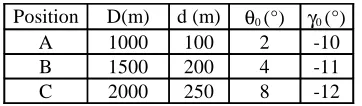
summarized in Table I and Fig. 2. For each set, D,d, and thus θ0 and γ0 are given. For each set, summed signals (21) are simulated in stable atmospheric conditions. The atmosphere parameters are derived from Fascode data for a continental climate, 30 km visibility.
Position D(m) d (m) θ0 (°) γ0 (°)
A 1000 100 2 -10
B 1500 200 4 -11
[image:5.612.87.268.132.185.2]C 2000 250 8 -12
[image:5.612.326.548.194.374.2]Table I – Geometric parameters of field observations
Figure 2 - Observation geometry
Values of γ0 are smaller than the half field of view, so that laser source is observed.
[image:5.612.46.300.217.314.2]For each of the three points of observation, in the case of a laser source placed at 200 m of altitude, the simulated signals are presented in Fig. 3.
Figure 3 - Simulated signals with Ta=16Ts=160ns (acquisition
time) and tm=4Ts=Ta/4=40ns (delay time of envelope max) .
value of SNR, two tm and position A.
Pd is equal to 1 for
γ
>0. The performances of detections are not very dependent on the delay (tm=Ta/4 or tm=3*Ta/4) between acquisition window and signal, in the case of optimal recovery (overlapping superior to 50%).Pfa has an instantaneous variation from 1 to 0 around
γ
for all snr values, in the case where the signal is not inacquisition window (tm< -Ta/4) . This property forces to choose
γ
always higher than 0 to ensure a very weak pfa.Figure 4 -Pd for tm=Ta/4 or tm=3*Ta/4 pfa :for tm<-Ta/4
[image:5.612.58.282.446.629.2]according snr=18dB and position A.
Fig. 5 makes it possible to determine the level
γ
optimal for a pd=99.9 according to SNR and simulated signals.γ
=1.8 is the optimal threshold which ensures a pd=99.9 and a pfa near to 0 for the three positions of laser source and snr near to 10dB.Figure 5 -
γ
maximum value ensuring pd=99.9% for tm=Ta/4 [image:5.612.326.549.500.678.2]This Bayesian method has performances much higher than the technique of detection per threshold. The latter gives results satisfying for position A only starting from snr of 40dB.
Detection and recognition algorithm 27 runs in line and processes into continuous permanent samples flow delivered by camera. Its computing power around 600 M Flops is adapted to current processing systems.
CONCLUSION
The model derived analytic formulas for computing, array sensor power of backscattered light incoming from a beam propagating in the atmosphere, has been developed in a 3D geometry.
Off-axis laser camera detection performances can so be calculated for different observation geometries and atmospheric conditions.
Using a generic sensor array, field trials is conducted for validating Bayesian detection algorithm. Simulation results allow to set correctly algorithm and optimise processing time.
The model is therefore able to predict Bayesian detection performance in many operational situations and can be extended to different cameras.
In the near future, the algorithm will be improve, and validate with signals bank based on many more geometric conditions and for very different atmospheric conditions.
REFERENCES
[1] B.H. Björkman, Apparatus for determining the path of a pulsed light beam, United States Patent, U.S. Philips Corporation, New York, 1987.
[2] D. V. Lindley, Introduction to probability and statistics from a Bayesian viewpoint I, II, Cambridge Univ. Press, 1965.