Abstract—This research assesses the performance of unreliable serial production lines having three simultaneous types of imbalance in terms of their mean operation times, coefficients of variation and buffer sizes. The lines were simulated with various line lengths, total buffer capacities, degrees of imbalance, and patterns of imbalance. Throughput, idle time and average buffer level data were gathered, analyzed and compared to a balanced line counterpart. It was found that an inverted bowl allocation of mean service times combined with a bowl configuration for both coefficients of variation and buffer sizes, resulted in higher throughput, whereas lower idle times were obtained from bowl assignments of mean processing times, coefficients of variation and buffer capacities. Furthermore, substantially lower average inventory levels were consistently achieved when utilizing a configuration of progressively higher mean service times and coefficients of variation in conjunction with assigning larger buffer capacities towards the end of the line.
Index Terms—Coefficient of variation imbalance, unequal mean operation times, uneven buffer capacity distribution, Unreliable production line.
I. INTRODUCTION
When setting up an un-paced serial production line, there are a number of issues to be considered if efficiency is to be enhanced. For instance, where to place operators who work at different speeds, or vary in the speed they work at, or where to keep unfinished items along the production line are just some of the problems facing the line manager.
The operators at each station along the line work at different average work times (MTs) for several reasons, some are personal, their physical capacity, their motivation and some are inherent to the task, it might be a complex task or just simply that the amount of work along the line just cannot be distributed evenly in terms of time. Therefore, the allocation of the operators along the line becomes an important consideration.
Not only do different operators work at different average speeds, the same person can vary in the rate at which he or
Manuscript received June 2, 2009.
S. Shaaban is with the ESC Rennes School of Business, Rennes, 35065, France (phone: +33(0) 299 54 63 31; fax: +33(0) 299 33 08 24; e-mail: [email protected]).
T. McNamara is with the ESC Rennes School of Business, Rennes, 35065, France (phone: +33(0) 299 54 63 63; fax: +33(0) 299 33 08 24; e-mail: [email protected]).
.
she works over the day for example. This can be for different reasons: fatigue, boredom and tasks that are complex or changing. One way of gauging this variation is to calculate the coefficient of variation (CV).
Another factor that needs thinking about is determining the size and location of the storage buffer spaces in between workstations where partly finished products are kept. In theory, an even distribution of buffer space along the line is the most effective. However, this is not always possible for technical reasons and a manager may have to distribute buffer capacity (BC) unevenly.
This paper is organized as follows. In sections 2 and 3 the relevant literature is reviewed and the research objectives are stated. Section 4 discusses the methodology and experimental design aspects. The simulation output data are exhibited and analysed in section 5. A summary and discussion of the findings, along with a set of conclusions, are presented in sections 6 and 7.
II. LITERATURE REVIEW
The research on unreliable, unbalanced flow lines can be broken down into the following categories:
A. Unreliable lines with unequal MTs:
[1] analysed a two-station line using a Markovian numerical method to predict the average number of pieces in the system, utilization rate of each station and throughput rate. [2] put forth a decomposition method for predicting the output of a production line having random MTs.
[3] studied Theory of Constraints (TOC) lines and found that positioning the constraint (the slowest or bottleneck station) at the first location minimizes flow time, work in process (WIP) and waiting times. Increasing protective capacity (the difference between the fastest and slowest stations) improves performance.
[4] observed that the location of the constraint station does not substantially influence line performance and that WIP exerts the greatest impact on cycle time, with higher WIP levels resulting in longer cycle times and a reduction in the effectiveness of protective capacity. As protective capacity is increased, cycle time decreases but at a diminishing rate. Increasing CV has a negative effect on line efficiency.
Unreliable Flow Lines with Jointly Unequal
Operation Time Means, Variabilities and Buffer
Sizes
B. Unreliable lines with uneven buffer capacities:
[5] developed a simple heuristic for determining the optimal allocation of buffers that maximizes throughput. Other authors (see [6] – [10]) offered a number of heuristic or optimization algorithms, sometimes incorporating simulation, for finding efficient buffer allocation with such objectives as output increase, or profit maximization. [11] presented two different algorithms; one addresses the problem of determining the minimum amount of buffers needed to maintain some predetermined production level (referred to as the ‘Primal’ problem), while the other seeks to maximize output, given a total amount of buffer capacity (referred to as the ‘Dual’ problem).
[12] focused on methods that minimize average WIP, while keeping a set throughput, subject to a fixed total buffer capacity. [13] developed heuristics for determining the smallest amount of buffer (termed ‘lean buffering’) needed to obtain throughput levels that are 85%, 90% and 95% of a theoretical maximum production rate. [14] derived analytical expressions for quantifying efficient buffer levels that are necessary for a minimum output rate
C. Unreliable lines with simultaneously unequal MTs and buffer sizes:
[15] proposed an algorithm for the optimal allocation of buffers in MT unbalanced lines. The solution method calculates the degree to which an increase in a unit of buffer raises line output. A number of other researchers developed a host of optimization and heuristic algorithms for the allocation of buffers in MT unbalanced lines in terms of maximizing profit or throughput (see [7], [10] and [16] – [23]).
[2] showed a decomposition method for predicting the output of a line having random MTs and unequal buffers. [24] developed an algorithm for the prediction of throughput rate.
D. Unreliable lines with combined unbalanced MTs and CVs:
[25] performed a series of simulation experiments for an unreliable two-stage queuing system having unequal MTs and CVs. They employed regression models to estimate the production rate and CV of the inter-departure rate for a work pieces.
[26] presented an efficient algorithm for computing the output of flow lines with generally distributed processing times, that are subject to downtime and scrapping. Their method explicitly considers the effects of simultaneous blocking and starving of stations.
III. MOTIVATION AND OBJECTIVES
This paper investigates the operating characteristics of unreliable production lines having three simultaneous sources of imbalance, namely by allowing both MTs and CVs to differ amongst the individual stations while distributing BCs unevenly along the buffers.
The motivation for undertaking this study is the relative lack of knowledge about the behaviour of such lines. The present paper aims to fill in many of the gaps in this area through the use of a more comprehensive and systematic investigation than hitherto attempted.
The main objectives of this investigation are:
• To assess various patterns of joint MT, CV and BC imbalance and attempt to identify the most promising ones.
• To compare the performance of such favourable patterns with that of a corresponding balanced line.
• To shed light on the characteristics of three performance measures for such lines, i.e. throughput, idle time and average buffer level
• To study the impacts of various line design variables on the dependent effectiveness measures.
IV. METHODOLOGY AND EXPEIMENTAL DESIGN Computer simulation was viewed as the most suitable tool for this study, since no mathematical method can currently assess the more realistic serial flow lines, typically reported with positively skewed operation times. The unbalanced line behaviour was studied using a ProModel Version 6 coded manufacturing simulation model.
A. Factorial Design
A full factorial design was deemed to be the most apt for the current study. For the specific line studied the independent variables were:
• Line length (number of stations), N. • Total buffer capacity for the line, TB. • Mean capacity of each buffer, MB. • CV value range.
• MT imbalance pattern • CV imbalance pattern. • BC imbalance pattern.
To depict more realistic processing times, a right shifted Weibull distribution was employed. [27] reported that this probability distribution closely describes the unpaced service times found in real practice.
B. Performance Measures
Three measures were used in this investigation: line throughput (TR), total idle time percentage (IT), i.e. the fraction of time that the line is inactive compared with total working time, and the average buffer level (ABL) for the whole line. Evidently, the study goals are to increase TR, reduce IT and ABL.
C. Simulation Run Parameters
To avoid having start-up data in the steady-state output, each simulation run was started with empty buffers and all collected statistics during the first 30,000 minutes warm up period were discarded.
reducing serial correlation to a negligible level. A trial procedure has established that the selected subrun length achieved minimal serial correlation values that were within the normally acceptable range of between – 0.20 and + 0.20 for computer simulations using ProModel software [28], leading to the conclusion that adjacent subruns were relatively independent.
In addition, in order to generate an identical event sequence for all the designs and highlight the contrast amongst the configurations, the same random number seed was used in all the experiments.
D. Failure and Repair Parameters
In unreliable lines the stations are subject to random mechanical failure and repair times. [29] found that in actual manufacturing systems an exponential distribution was the most representative probability function for both the mean time before failure (MTBF) and mean time to repair (MTTR). Furthermore, MTBF and MTTR were set at 100 and 10 minutes, respectively. These were the same values used by [16] and [30].
E. Model Assumptions
Several relatively standard assumptions for the type of lines being studied were made. These are that no defective items are made, only one type of product is manufactured, no changeover time was needed, the time to move work pieces in and out of the buffers is negligible, the first station never suffers from starving delays, and the last station is never blocked.
F. Specific Design Features
• Number of stations (N): N values of 5 and 8 were specified.
• Total buffer capacity (TB) in units: TB values of 8, 24 (for N = 5), and 14, 42 (for N = 8) were selected, giving rise to mean buffer capacity (MB) of 2 & 6 for both N = 5 and 8.
• % Degree of imbalance (DI), i.e. the degree of difference in the speeds between successive stations in the line: DI values of 2% (slight), 5%, and 12% (relatively high) were chosen.
• MT imbalance configuration: The work stations were arranged in four different patterns according to their mean operation times:
• Decreasing order (\) – going from slowest to fastest operators.
• Increasing order (/) – going from fastest to slowest operators.
• An inverted bowl (
٨
) – the slowest operators
positioned in the middle.• A bowl arrangement (V) - the fastest operators positioned in the middle.
•
CV allocation pattern: four patterns were considered: • P1: the stations having high variability are assignedto the beginning of the line - a CV decreasing order (\).
• P2: concentrating the stations with high variability towards the end of the line - an increasing CV order (/).
• P3: the most variable stations are allocated to the line's centre - an inverted bowl arrangement (Λ). • P4: concentrating the steadiest stations towards the
line centre - a bowl arrangement (V).
• TB allocation arrangement: four patterns were investigated:
• Concentrating buffer capacity nearer the beginning of the line (P1) - a generally decreasing order (\) of BC.
• Concentrating buffer capacity nearer the end of the line (P2) - a generally increasing order (/) of BC. • Concentrating buffer capacity nearer the middle of
the line (P3) - a generally inverted bowl-shaped (٨) sequence of BC. .
• Smaller BC amounts are positioned towards the centre (P4) – a generally bowl - (V) looking configuration.
Overall, a total of 768 simulation experiments (2 * 2 * 3 * 4 * 4 * 4) were needed inthis investigation.
Figures 1 to 3 listed below show the CV and BC imbalance patterns employed:
Line Length (N) Pattern (P) of
Unbalanced CVs 5 8
P1 VMMMS VVMMMMSS
P2 SMMMV SSMMMMVV
P3 MVVVS MMVVVVSS
P4 VSSSM VVSSSSMM
S = relatively steady CV (CV = 0.08) M = medium CV (CV = 0.27)
V = relatively more variable CV (CV = 0.50) Fig. 1: Unbalanced CV patterns
[image:3.595.308.530.394.621.2]
Fig. 2: Unequal buffer size patterns N = 5
Line Length (N) 5
Mean Buffer
Capacity (MB) 2 6
P1 4, 2, 1, 1 12, 6, 3, 3 P2 1, 1, 2, 4 3, 3, 6, 12 P3 1, 3, 3, 1 3, 9, 9, 3 Pattern
of Buffer Capacity Imbalance
(Pi) P4 3, 1, 1, 3 9, 3, 3, 9 Total Buffer
Line Length
(N) 8
Mean Buffer
Capacity (MB) 2 6
P1 6, 2, 2, 1, 1, 1, 1 18, 6, 6, 3, 3, 3, 3 P2 1, 1, 1, 1, 6, 2, 2 3, 3, 3, 3, 18, 6, 6 P3 1, 1, 4, 4, 2, 1, 1 3, 3, 12, 12, 6, 3, 3 Pattern
of Buffer Capacity Imbalanc
e (Pi)
P4 4, 2, 1, 1, 3, 2, 1 12, 6, 3, 3, 9, 6, 3 Total Buffer
Capacity (TB) 14 42
Fig. 3: Unequal buffer size patterns N = 8
V. RESULTS
A. Ranking of Throughput Patterns and Comparison with the Balanced Line
Tables 1 through 4 below exhibit TR data:
Table I: TR data for the best, good, worst patterns and a
balanced line N = 5, MB = 2
[image:4.595.42.271.61.232.2]Table II: TR data for the best, good, worst patterns and a balanced line N = 5, MB = 6
[image:4.595.311.539.262.389.2]Table III: TR data for the best, good, worst patterns and a balanced line N = 8, MB = 2
Table IV: TR data for the best, good, worst patterns and a balanced line N = 8, MB = 6
Mean Buffer Capacity (MB) 6
Pattern %DI Ranking
MT CV BC 2 5 12
Best /\ V V 0.837 0.851 0.818
Good / V V 0.849 0.835 0.778
Worst / /\ \ 0.795 0.786 0.776 Unreliable Balanced Line 0.851
From tables 1 through 4 the following findings were made: • The most superior TR pattern can be considered as the
combination of an inverted bowl MT arrangement, along with a CV and BC bowl configurations, i.e. the slowest and steadiest workers are positioned in the middle with more buffers allocated to the front and end of the line. • An increasing MT allocation, combined with a bowl
shape for both CV and BC is also a good pattern. • The worst pattern is an ascending MT order, in
conjunction with an inverted CV bowl and a decreasing BC sequence.
• A decreasing MT sequence coupled with an inverted CV bowl pattern provides consistently poor TR results when mixed with either an ascending or a bowl BC allocation. The same is true for an increasing MT shape in
association with an inverted CV bowl configuration and a descending or inverted bowl BC assignment.
B. Effects of the Design Variables on Throughput and Comparison with the Balanced Line
For the best pattern determined, the following relationships hold:
• As N goes up, TR decreases. • When MB rises, TR increases.
• Increasing N reduces the advantage of the best pattern over the unreliable balanced line.
Mean Buffer Capacity (MB) 2
Pattern %DI Ranking
MT CV BC 2 5 12
Best /\ V V 0.815 0.802 0.785
Good / V V 0.807 0.802 0.774
Worst / /\ \ 0.732 0.720 0.704 Unreliable Balanced Line 0.800
Mean Buffer Capacity (MB) 6
Pattern %DI Ranking
MT CV BC 2 5 12
Best /\ V V 0.854 0.858 0.846
Good / V V 0.851 0.856 0.805
Worst / /\ \ 0.796 0.799 0.765 Unreliable Balanced Line 0.850
Mean Buffer Capacity (MB) 2
Pattern %DI Ranking
MT CV BC 2 5 12
Best /\ V V 0.778 0.773 0.770 Good / V V 0.778 0.776 0.725 Worst / /\ \ 0.601 0.690 0.693
C. Ranking of Idle Time Patterns and Comparison with the Balanced Line
[image:5.595.43.302.143.267.2]Tables 5 through 8 below show %IT data:
Table V: %IT data for the best, good, worst patterns and a balanced line N = 5, MB = 2
Mean Buffer Capacity (MB) 2
Pattern %DI Ranking
MT CV BC 2 5 12
Best V V V 19.408 18.942 20.416
Good / V V 19.162 19.456 22.326
[image:5.595.42.296.319.440.2]Worst / /\ \ 26.216 27.492 29.984 Unreliable Balanced Line 19.654
Table VI: %IT data for the best, good, worst patterns and a balanced line N = 5, MB = 6
Table VII: %IT data for the best, good, worst patterns and a balanced line N = 8, MB = 2
Table VIII: %IT data for the best, good, worst patterns and a balanced line N = 8, MB = 6
Looking at tables 5 through 8 the most important findings are as follows:
• The best IT pattern is where MT, CV and BC are all distributed in a bowl fashion. That is to say, the fastest and least variable workers are placed in the middle of the line while placing most BC in the front and back of the line
• An increasing MT sequence, in conjunction with a bowl arrangement for both CV and BC is a good pattern. • The worst pattern is an ascending order MT allocation,
blended with an inverted bowl shaped CV positioning and a descending BC arrangement.
• The good and worst patterns in regards to IT turned out to be exactly the same as those obtained for TR. • An arrangement of decreasing or increasing MTs and a
CV inverted bowl allotment, combined with either ascending or bowl BC configurations consistently generate unfavourable IT results.
D. Effects of the Design Variables on Idle Time and Comparison with the Balanced Line:
The following relationships were observed for the best pattern:
• As MB rises, IT declines.
• When N increases, the superiority of the best pattern over the balanced line goes down.
E. Ranking of ABL Patterns and Comparison with the Balanced Line
[image:5.595.43.294.490.744.2]Tables 9 through 12 summarise the ABL data.
Table IX: ABL data for the best, 2nd best, some good, worst patterns and a balanced line N = 5, MB = 2
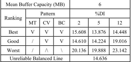
Mean Buffer Capacity (MB) 6
Pattern %DI Ranking
MT CV BC 2 5 12
Best V V V 15.608 13.876 14.448
Good / V V 14.610 14.224 19.016
Worst / /\ \ 20.136 19.888 23.142 Unreliable Balanced Line 14.636
Mean Buffer Capacity (MB) 2
Pattern %DI Ranking
MT CV BC 2 5 12
Best V V V 22.758 22.368 22.636
Good / V V 22.481 22.831 27.560
Worst / /\ \ 29.920 31.061 30.979
Balanced Line 20.835
Mean Buffer Capacity (MB) 6
Pattern %DI Ranking
MT CV BC 2 5 12
Best V V V 15.481 15.049 18.054 Good / V V 15.141 17.128 22.290 Worst / /\ \ 20.900 21.666 23.069
Balanced Line 15.246
Mean Buffer Capacity (MB) 2
Pattern %DI Ranking
MT CV BC 2 5 12
Best \ \ / 0.475 0.393 0.280
Table X: ABL data for the best, 2nd best, some good, worst patterns and a balanced line N = 5, MB = 6
Mean Buffer Capacity
(MB) 6
Pattern %DI Ranking
MT CV BC 2 5 12
Best \ \ / 0.966 0.848 0.664
2nd Best \ V / 1.180 0.924 0.670
Good \ V /\ 1.403 1.517 0.603
Good \ \ /\ 2.185 0.988 0.723
Worst / / \ 4.781 4.816 5.397
[image:6.595.44.266.470.624.2]Unreliable Balanced Line 2.782
Table XI: ABL data for the best, 2nd best, some good, worst patterns and a balanced line N = 8, MB = 2
Mean Buffer Capacity
(MB) 2
Pattern %DI Rankin
g MT CV BC 2 5 12
Best \ \ / 0.446 0.397 0.271 2nd Best \ V / 0.485 0.397 0.269
Good \ V /\ 0.493 0.432 0.310 Good \ \ /\ 0.616 0.448 0.310 Worst / / \ 1.618 1.631 1.741 Unreliable Balanced Line 1.056
Table XII: ABL data for the best, 2nd best, some good, worst patterns and a balanced line N = 8, MB = 6 Mean Buffer Capacity (MB) 6
Pattern %DI Ranking
MT CV BC 2 5 12
Best \ \ / 1.034 0.925 0.672 2nd Best \ V / 1.006 0.841 0.699
Good \ V /\ 1.184 1.117 0.549 Good \ \ /\ 1.236 0.949 0.737 Worst / / \ 4.924 5.087 5.324 Unreliable Balanced Line 3.172
From tables 9 through 12 the following can be noted: • The best ABL pattern is the combination of descending
MT and CV orders and an ascending BC sequence, i.e. as one moved down the line the stations got faster and less variable with increasing amounts of B being allocated.
• The second best pattern is a decreasing MT order, coupled with bowl CV and increasing BC allocations, respectively.
• Other good patterns are a decreasing sequence of MT, accompanied by an inverted bowl BC shape and either a CV bowl or a CV descending order.
• The least favourable pattern is increasing MT and CV arrangements, accompanied by a descending BC order. • The best and a number of other patterns provided
reduced ABL at all N, MB and DI levels studied. • The advantage of a decreasing MT order can be clearly
seen in the best, 2nd best, good and other favourable patterns.
F. The Effects of the Design Variables on ABL and Comparison with the Balanced Line
For the best unbalanced pattern found, the following relationships were seen:
• ABL becomes larger when MB is increased. • As DI is increased, ABL falls.
• The best and a number of other favourable patterns have substantially lower ABL values than those of the balanced line under all the conditions simulated. • When N, MB, or DI go up, the advantage in ABL of the
best unbalanced line over the control increases
G. Savings produced by the Best TR, IT and ABL Patterns From the above it can be seen that unbalancing the lines can provide real improvements over a balanced line if they are designed properly. Tables 13 - 15 provide summaries of the % change in the best pattern’s TR, IT and ABL over a balanced line (control) counterpart:
Table XIII: % change in the best pattern’s TR over the control
N = 5 N = 8
MB % DI % Change MB % DI % Change
2 2 1.81%* 2 2 -2.26%
2 5 0.25% 2 5 -2.83% 2 12 -1.88% 2 12 -3.21% 6 2 0.47% 6 2 -1.59% 6 5 0.94% 6 5 0.00% 6 12 -0.47% 6 12 -3.88% (-) Indicates a deterioration in TR
* Best saving obtained
Table XIV: % change in the best pattern’s IT over the control
N = 5 N = 8
MB % DI % Change MB % DI % Change 2 2 -1.25% 2 2 9.23% 2 5 -3.62% 2 5 7.36% 2 12 3.88% 2 12 8.65% 6 2 6.64% 6 2 1.54%
6 5 -5.19%* 6 5 -1.30%
6 12 -1.28% 6 12 18.41% (-) Indicates a saving in IT
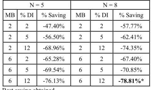
[image:6.595.302.527.596.741.2]Table XV: % savings in the best pattern’s ABL over the control
N = 5 N = 8
MB % DI % Saving MB % DI % Saving 2 2 -47.40% 2 2 -57.77% 2 5 -56.50% 2 5 -62.41% 2 12 -68.96% 2 12 -74.35% 6 2 -65.28% 6 2 -67.40% 6 5 -69.54% 6 5 -70.85%
6 12 -76.13% 6 12 -78.81%*
* Best saving obtained
From tables 13 – 15, it can be observed that:
• The greatest saving in TR (1.81%) was achieved via having a 5-station unbalanced line with MB = 2 and DI = 2%.
• A line having 5 stations with MB = 6 and DI = 5, resulted in the highest advantage (over 5% saving).
• A significant reduction in ABL (almost 79%) was obtained for an 8-station line with MB = 6 and DI = 12%.
VI. SUMMARY
It was found that when the fastest and steadiest workers are placed in the middle of the line, while placing most buffer capacity in the front and back of the line resulted in higher throughput and levels than those arrived at by a balanced line counterpart.
In addition, lower idle time values were obtained by positioning the fastest and least variable workers in the middle of the line, combined with the allocation of most buffer capacity at the beginning and end of the line. Furthermore, it was observed that substantially lower average inventory levels as compared to a balanced line were consistently obtained when utilizing a configuration of progressively faster and less variable stations, in conjunction with larger buffer sizes being assigned towards the end of the line.
The following main relationships were discerned from analysing the data:
• As N goes up, TR goes down.
• When MB rises, both TR and ABL increase, but IT declines.
• ABL falls as DI is increased.
• Increasing N will decrease the superiority in both TR and IT of the best pattern in comparison with an unreliable balanced line.
• When N, MB, or DI increases, the advantage in ABL of the best configuration increases.
• The best pattern as well as other favourable patterns exhibit substantially lower ABL values than those of the unreliable balanced line for all the situations simulated.
VII. CONCLUSION
Since a nominally balanced line in terms of MT and CV, with evenly distributed buffers remains an unlikely goal for manually operated lines, then unbalancing the line in the correct manner can give better results almost free of charge, as savings can be reaped while assigning existing operators to the same stations at no extra labour or capital investment. This study has demonstrated that none of the patterns considered simultaneously brought about high TR, low IT, or reduced ABL levels. Whether a line designer views an increased TR (or a decreased IT) as more advantageous than a low ABL, will partly depend on inventory keeping and buffer space costs relative to lost production.
A line manager, therefore will have to make decisions as to where the greatest benefits can be reaped. It may be to reduce idle time, should it be costly, for instance in an industry where demand is high and operators are working full out, such as on the production lines in consumer goods (e.g. toys, shoes and office supplies), or where manpower is expensive. In these cases, where any idle time leads to great expense, the best or other favourable jointly unbalanced MT, CV and BC designs will be selected to get the largest possible idle time reduction, or throughput rise.
It may be, however, that the principal aim is lean buffering, as in the automotive and electronics industry, where
just-in-time management requires it. Here, the best or some other advantageous unbalanced patterns which bring average buffer levels down would be the most appropriate.
As with all research of this nature, it should be emphasized, though, that only a limited number of configurations among an almost infinite number of alternatives for unbalancing the line were examined. Therefore, if imbalance was made in the wrong way, it could lead to adverse performance, i.e. increases in average buffer levels or idle times, or declines in throughput rates.
In spite of this, however, the scale of the potential reductions in throughput (nearly 1.8%), idle time (over 5%), and average buffer level (some 79%), when calculated over the working lifespan of a production line means that purposely unbalancing the buffer sizes and operators with different mean service times and modes of variability could lead to real benefits for the manufacturer, and so might be a strategy to take into account when designing the production line.
REFERENCES
[1] T. Altiok, “Production lines with phase-type operation repair times and finite buffers,” International Journal of Production Research, vol. 23, no. 3, 1985, pp. 489 - 498.
[2] Y. F. Choong, and S. B. Gershwin, “A decomposition method for the approximate evaluation of capacitated transfer lines with unreliable machines and random processing times,” IIE Transactions, vol. 19, no. 2, 1987, pp.150 -1 59.
[3] S. K. Kadipasaoglu, W. Xiang, S. F. Hurley, and B. M. Khumawala, “A study on the effects of the extent and location of protective capacity in flow systems,” International Journal of Production Economics, vol. 63, 2000, pp. 217 - 228.
[4] W. L. Sloan, “A study on the effects of protective capacity on cycle time in serial production lines,” M.Sc. Thesis, Mississippi State University, 2001.
[5] F. S. Hillier, and K. C. So, “The effect of machine breakdowns and inter-stage storage on the performance of production line systems,” International Journal of Production Research, vol. 29, no. 10, 1981, pp. 2043 - 2055.
[6] A. A. Bulgak, P. D. Diwan, and B. Inozu, “Buffer size optimization in asynchronous assembly systems using genetic algorithms,” Computers and Industrial Engineering, vol. 28, no. 2, 1995, pp. 309 - 322.
[7] G. A. Vouros, and H. T. Papadopoulos, “Buffer allocation in unreliable production lines using a knowledge based system,” Computers and Operations Research, vol. 25, no. 12, 1998, pp. 1055 - 1067.
[8] H. T. Papadopoulos, and M. I. Vidalis, “Optimal buffer allocation in short μ-balanced unreliable production lines,” Computer and Industrial Engineering, vol. 37, 1999, pp. 691 - 710. [9] S. Helber, “Cash-flow-orientated buffer allocation in stochastic flow lines,” International Journal of Production Management, vol. 39, no. 14, 2001, pp. 3061 – 3083. [10] N. Nahas, D. Ait-Kadi, and M. Nourelfath, “A new approach for buffer allocation in unreliable production lines,” International Journal of Production Economics, vol. 103, 2006, pp. 873 - 881. [11] S. B. Gershwin, and J. E. Schor, “Efficient algorithms for buffer space allocation,” Annals of Operations Research, vol. 93, 2000, pp. 117 -144.
[12] S. Kim, and H. J. Lee, “Allocation of buffer capacity to minimize average work-in-process,” Production Planning & Control, vol. 12, no. 7, 2001, pp. 706 – 716.
[13] E. Enginarlar, J. Li, S. M. Meerkov, and R. Q. Zhang, “Buffer capacity for accommodating machine downtime in serial production lines,” International Journal of Production Research, vol. 40, no. 3, 2002, pp. 601 - 624.
[14] E. Enginarlar, J. Li, and S. M. Meerkov, “Lean buffering in serial production lines with non-exponential machines,” OR Spectrum, vol. 27, 2005, pp. 195 - 219.
[15] Y. C. Ho, M. A. Eyler, and T. T. Chien, “A gradient technique for general buffer storage design in a production line,” International Journal of Production Research, vol. 17, no. 6, 1979, pp. 557 - 580. [16] T. Altiok, and S. Stidham, “The allocation of inter-stage buffer capacities in production lines,” IIE Transactions, vol. 15, no. 4, 1983, pp. 292 – 299.
[17] D. Seong, S. Y. Chang, and Y. Hong, “Heuristic algorithms for buffer allocation in a production line with unreliable machines,” International Journal of Production Research, vol. 33, no. 7, 1995, pp. 1989 - 2005.
[18] G. Gürkan, “Simulation optimization of buffer allocation in production lines with unreliable machines,” Annals of Operations Research, vol. 93, nos. 1 - 4, 2000, pp.177 - 216.
[19] H. T. Papadopoulos, and M. I. Vidalis, “A heuristic algorithm for the buffer allocation in unreliable unbalanced production lines,” Computers & Industrial Engineering, vol. 41, 2001, pp.261 - 277. [20] A. Dolgui, A. Eremeev, A. Kolokolov, and V. Sigaev, “A genetic algorithm for the allocation of buffer storage capacities in a production line with unreliable machines,” Journal of Mathematical Modelling and Algorithms, vol. 1, 2002, pp. 89 - 104.
[21] L. Shi, and S. Men, “Optimal buffer allocation in production lines,” IIE Transactions, vol. 35, 2003, pp.1 – 10.
[22] M. Nourelfath, N. Nahas, and D. Ait-Kadi, “Optimal design of series production lines with unreliable machines and finite buffers,” Journal of Quality Maintenance Engineering, Vol. 11, No. 2, 2005, pp. 121 - 138.
[23] I. Sabuncuoglu, E. Erel, and Y. Gocgun, “Analysis of serial production lines: characterisation study and a new heuristic procedure for optimal buffer allocation,” International Journal of Production Research, vol.44, no. 13, 2006, pp. 2499 - 2523. [24] C. Heavey, H. T. Papadopoulos, and J. Browne, “The throughput of multistation unreliable production lines,” European Journal of Operational Research, vol. 68, 1993, pp. 69 - 89.
[25] W. M. Chow, “Buffer capacity analysis for sequential production lines with variable process times,” International Journal of Production Research, vol. 25, no. 8, 1987, pp. 1183 - 1196. [26] H. Tempelmeier, and M. Burger, “Performance evaluation of unbalanced flow lines with general distributed processing times, failures and imperfect production,” IIE Transactions, vol. 33, 2001, pp. 293 - 302.
[27] N. Slack, “Work time distributions in production system modelling,” Research Paper, Oxford Centre for Management Studies, 1982. [28] C. Harrell, B. K. Ghosh, and R. O. Bowden, R. O. Simulation Using ProModel. New York, NY: McGraw Hill, 2004.
[29] R. R. Inman, “Empirical evaluation of exponential and independence assumptions in queuing models of manufacturing systems,” Production and Operations Management, Vol. 8, No. 4, 1999, pp. 409 - 432.