Generalizing and Hybridizing Count-based and Neural Language Models
Graham Neubig† and Chris Dyer‡ †Carnegie Mellon University, USA ‡Google DeepMind, United Kingdom
Abstract
Language models (LMs) are statistical mod-els that calculate probabilities over sequences of words or other discrete symbols. Currently two major paradigms for language model-ing exist: count-basedn-gram models, which
have advantages of scalability and test-time speed, and neural LMs, which often achieve superior modeling performance. We demon-strate how both varieties of models can be uni-fied in a single modeling framework that de-fines a set of probability distributions over the vocabulary of words, and then dynamically calculates mixture weights over these distri-butions. This formulation allows us to create novel hybrid models that combine the desir-able features of count-based and neural LMs, and experiments demonstrate the advantages of these approaches.1
1 Introduction
Language models (LMs) are statistical models that, given a sentence wI
1 := w1, . . . , wI, calculate its
probabilityP(wI1). LMs are widely used in
applica-tions such as machine translation and speech recog-nition, and because of their broad applicability they have also been widely studied in the literature. The most traditional and broadly used language model-ing paradigm is that of count-based LMs, usually smoothed n-grams (Witten and Bell, 1991; Chen
1Work was performed while GN was at the Nara Institute of Science and Technology and CD was at Carnegie Mellon Uni-versity. Code and data to reproduce experiments is available at
http://github.com/neubig/modlm
and Goodman, 1996). Recently, there has been a fo-cus on LMs based on neural networks (Nakamura et al., 1990; Bengio et al., 2006; Mikolov et al., 2010), which have shown impressive improvements in performance over count-based LMs. On the other hand, these neural LMs also come at the cost of in-creased computational complexity at both training and test time, and even the largest reported neural LMs (Chen et al., 2015; Williams et al., 2015) are trained on a fraction of the data of their count-based counterparts (Brants et al., 2007).
In this paper we focus on a class of LMs, which we will call mixture of distributions LMs (MODLMs;§2). Specifically, we define MODLMs
as all LMs that take the following form, calculat-ing the probabilities of the next word in a sentence wi given preceding context c according to a
mix-ture of several component probability distributions Pk(wi|c):
P(wi|c) = K
X
k=1
λk(c)Pk(wi|c). (1)
Here, λk(c) is a function that defines the mixture
weights, with the constraint that PK
k=1λk(c) = 1
for allc. This form is not new in itself, and widely
used both in the calculation of smoothing coeffi-cients forn-gram LMs (Chen and Goodman, 1996), and interpolation of LMs of various varieties (Je-linek and Mercer, 1980).
The main contribution of this paper is to demon-strate that depending on our definition ofc, λk(c),
andPk(wi|c), Eq. 1 can be used to describe not only n-gram models, but also feed-forward (Nakamura et al., 1990; Bengio et al., 2006; Schwenk, 2007) and
recurrent (Mikolov et al., 2010; Sundermeyer et al., 2012) neural network LMs (§3). This observation
is useful theoretically, as it provides a single mathe-matical framework that encompasses several widely used classes of LMs. It is also useful practically, in that this new view of these traditional models allows us to create new models that combine the desirable features ofn-gram and neural models, such as:
neurally interpolatedn-gram LMs (§4.1), which learn the interpolation weights of n-gram models using neural networks, and
neural/n-gram hybrid LMs (§4.2), which add a count-basedn-gram component to neural mod-els, allowing for flexibility to add large-scale external data sources to neural LMs.
We discuss learning methods for these models (§5)
including a novel method of randomly dropping out more easy-to-learn distributions to prevent the pa-rameters from falling into sub-optimal local minima. Experiments on language modeling benchmarks (§6) find that these models outperform baselines in terms of performance and convergence speed.
2 Mixture of Distributions LMs
As mentioned above, MODLMs are LMs that take the form of Eq. 1. This can be re-framed as the fol-lowing matrix-vector multiplication:
p|c=Dcλ|c,
wherepcis a vector with length equal to vocabulary
size, in which the jth elementpc,j corresponds to P(wi=j|c),λcis a sizeKvector that contains the
mixture weights for the distributions, andDcis aJ
-by-K matrix, where element dc,j,k is equivalent to
the probabilityPk(wi = j|c).2 An example of this
formulation is shown in Fig. 1.
Note that all columns in Drepresent probability distributions, and thus must sum to one over the J words in the vocabulary, and that all λ must sum
to 1 over theK distributions. Under this condition, the vectorpwill represent a well-formed probability
distribution as well. This conveniently allows us to
2We omit the subscriptcwhen appropriate.
Probabilitiesp| Coefficientsλ|
z}|{ z}|{
p1
=
d1,1 d1,2 · · · d1,K λ1
p2 d2,1 d2,2 · · · d2,K λ2
... ... ... ... ... ...
pJ dJ,1 dJ,2 · · · dJ,K λK
| {z }
Distribution matrixD
Figure 1: MODLMs as linear equations
calculate the probability of a single wordwi =jby
calculating the product of thejth row ofDcandλ|c
Pk(wi =j|c) =dc,jλ|c.
In the sequel we show how this formulation can be used to describe several existing LMs (§3) as well as several novel model structures that are more power-ful and general than these existing models (§4).
3 Existing LMs as Linear Mixtures
3.1 n-gram LMs as Mixtures of Distributions First, we discuss how count-based interpolated n -gram LMs fit within the MODLM framework.
Maximum likelihood estimation: n-gram mod-els predict the next word based on the previousN-1 words. In other words, we set c = wii−−1N+1 and calculateP(wi|wii−−N1+1). The maximum-likelihood
(ML) estimate for this probability is
PM L(wi|wii−−N1+1) =c(wii−N+1)/c(wii−−1N+1), wherec(·)counts frequency in the training corpus.
Interpolation: Because ML estimation as-signs zero probability to word sequences where c(wii−N+1) = 0, n-gram models often interpolate the ML distributions for sequences of length 1 toN. The simplest form is static interpolation
P(wi|wii−−1n+1) = N
X
n=1
λS,nPM L(wi|wii−−1n+1). (2)
λS is a vector where λS,n represents the weight
put on the distributionPM L(wi|wii−−1n+1). This can
Probabilitiesp| Heuristic interp. coefficientsλ|
z}|{ z}|{
p1
=
d1,1 d1,2 · · · d1,N λ1
p2 d2,1 d2,2 · · · d2,N λ2
... ... ... ... ... ...
pJ dJ,1 dJ,2 · · · dJ,N λN
| {z }
Count-based probabilitiesPC(wi=j|wii−−n1+1) (a) Interpolatedn-grams as MODLMs
Probabilitiesp| Result of softmax(NN(c))
z}|{ z}|{
p1
=
1 0 · · · 0 λ1
p2 0 1 · · · 0 λ2
... ... ... ... ... ...
pJ 0 0 · · · 1 λJ
| {z }
J-by-J identity matrixI
[image:3.612.88.518.67.181.2](b) Neural LMs as MODLMs
Figure 2: Interpretations of existing models as mixtures of distributions
Static interpolation can be improved by calcu-lating λ(c) dynamically, using heuristics based on
the frequency counts of the context (Good, 1953; Katz, 1987; Witten and Bell, 1991). These meth-ods define a context-sensitive fallback probability α(wii−−1n+1)for ordernmodels, and recursively cal-culate the probability of the higher order models from the lower order models:
P(wi|wii−−n1+1) =α(wii−−1n+1)P(wi|wii−−n1+2)+ (1−α(wii−−n1+1))PM L(wi|wii−−1n+1). (3) To express this as a linear mixture, we con-vert α(wii−−n1+1) into the appropriate value for
λn(wii−−N1+1). Specifically, the probability assigned to eachPM L(wi|wii−−n1+1)is set to the product of the
fallbacksαfor all higher orders and the probability of not falling back (1−α) at the current level:
λn(wii−−N1+1) = (1−α(wii−−n1+1)) N
Y
˜ n=n+1
α(wii−−1˜n+1).
Discounting: The widely used technique of dis-counting (Ney et al., 1994) defines a fixed discount dand subtracts it from the count of each word before calculating probabilities:
PD(wi|wii−−n1+1) = (c(wii−n+1)−d)/c(wii−−n1+1). Discounted LMs then assign the remaining probabil-ity mass after discounting as the fallback probabilprobabil-ity
βD(wii−−n1+1) =1− J
X
j=1
PD(wi =j|wii−−1n+1), P(wi|wii−−n1+1) =βD(wii−−1n+1)P(wi|wii−−n1+2)+
PD(wi|wii−−n1+1). (4)
In this case,PD(·)does not add to one, and thus
vi-olates the conditions for MODLMs stated in§2, but it is easy to turn discounted LMs into interpolated LMs by normalizing the discounted distribution:
PN D(wi|wii−−n1+1) =
PD(wi|wii−−1n+1)
PJ
j=1PD(wi =j|wii−−1n+1) ,
which allows us to replaceβ(·)forα(·)andPN D(·)
forPM L(·)in Eq. 3, and proceed as normal.
Kneser–Ney (KN; Kneser and Ney (1995)) and Modified KN (Chen and Goodman, 1996) smooth-ing further improve discounted LMs by adjustsmooth-ing the counts of lower-order distributions to more closely match their expectations as fallbacks for higher or-der distributions. Modified KN is currently the de-facto standard in n-gram LMs despite occasional improvements (Teh, 2006; Durrett and Klein, 2011), and we will express it asPKN(·).
3.2 Neural LMs as Mixtures of Distributions In this section we demonstrate how neural network LMs can also be viewed as an instantiation of the MODLM framework.
Feed-forward neural network LMs: Feed-forward LMs (Bengio et al., 2006; Schwenk, 2007) are LMs that, like n-grams, calculate the prob-ability of the next word based on the previous words. Given context wii−−N1+1, these words are converted into real-valued word representation vec-torsrii−−1N+1, which are concatenated into an over-all representation vector q = ⊕(rii−−1N+1), where ⊕(·) is the vector concatenation function. qis then run through a series of affine transforms and non-linearities defined as function NN(q) to obtain a
net-Probabilitiesp| Result of softmax(NN(c))
z}|{ z}|{
p1
=
d1,1 d1,2 · · · d1,N λ1
p2 d1,2 d2,2 · · · d2,N λ2
... ... ... ... ... ...
pJ dJ,1 dJ,2 · · · dJ,N λN
| {z }
Count-based probabilitiesPC(wi=j|wii−−1n+1) (a) Neurally interpolatedn-gram LMs
Probabilitiesp| Result of softmax(NN(c))
z}|{ z}|{
p1
=
d1,1 · · · d1,N 1 · · · 0 λ1
p2 d2,1 · · · d2,N 0 · · · 0 λ2
... ... ... ... ... ... ... ...
pJ dJ,1 · · · dJ,N 0 · · · 1 λJ+N
| {z }
Count-based probabilities andJ-by-Jidentity matrix
[image:4.612.82.536.68.181.2](b) Neural/n-gram hybrid LMs
Figure 3: Two new expansions ton-gram and neural LMs made possible in the MODLM framework
work with a tanh non-linearity we can define
NN(q) := tanh(qWq+bq), (5)
where Wq and bq are weight matrix and bias
vec-tor parameters respectively. Finally, the probabil-ity vectorpis calculated using the softmax function p=softmax(hWs+bs), similarly parameterized.
As these models are directly predictingpwith no
concept of mixture weightsλ, they cannot be
inter-preted as MODLMs as-is. However, we can per-form a trick shown in Fig. 2b, not calculatingp
di-rectly, but instead calculating mixture weightsλ =
softmax(hWs +bs), and defining the MODLM’s
distribution matrix D as a J-by-J identity matrix. This is equivalent to defining a linear mixture of J Kroneckerδjdistributions, thejth of which assigns
a probability of 1 to wordj and zero to everything else, and estimating the mixture weights with a neu-ral network. While it may not be clear why it is use-ful to define neural LMs in this somewhat round-about way, we describe in§4 how this opens up pos-sibilities for novel expansions to standard models.
Recurrent neural network LMs: LMs using recurrent neural networks (RNNs) (Mikolov et al., 2010) consider not the previous few words, but also maintain a hidden state summarizing the sentence up until this point by re-defining the net in Eq. 5 as
RNN(qi) := tanh(qiWq+hi−1Wh+bq),
whereqi is the current input vector andhi−1is the hidden vector at the previous time step. This allows for consideration of long-distance dependencies be-yond the scope of standardn-grams, and LMs using RNNs or long short-term memory (LSTM) networks (Sundermeyer et al., 2012) have posted large im-provements over standardn-grams and feed-forward
models. Like feed-forward LMs, LMs using RNNs can be expressed as MODLMs by predictingλ
in-stead of predictingpdirectly.
4 Novel Applications of MODLMs
This section describes how we can use this frame-work of MODLMs to design new varieties of LMs that combine the advantages of both n-gram and neural network LMs.
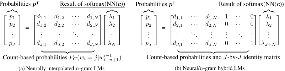
4.1 Neurally Interpolatedn-gram Models The first novel instantiation of MODLMs that we propose is neurally interpolated n-gram models, shown in Fig. 3a. In these models, we setDto be the same matrix used inn-gram LMs, but calculateλ(c)
using a neural network model. As λ(c) is learned
from data, this framework has the potential to allow us to learn more intelligent interpolation functions than the heuristics described in §3.1. In addition, because the neural network only has to calculate a softmax overN distributions instead of J vocabu-lary words, training and test efficiency of these mod-els can be expected to be much greater than that of standard neural network LMs.
Within this framework, there are several design decisions. First, how we decideD: do we use the maximum likelihood estimatePM Lor KN estimated
distributionsPKN? Second, what do we provide as
input to the neural network to calculate the mixture weights? To provide the neural net with the same information used by interpolation heuristics used in traditional LMs, we first calculate three features for each of theN contextswii−−1n+1: a binary feature in-dicating whether the context has been observed in the training corpus (c(wii−−1n+1) > 0), the log
zero for unobserved contexts), and the log frequency of the number of unique words following the context (log(u(wii−−1n+1))or likewise zero). When using
dis-counted distributions, we also use the log of the sum of the discounted counts as a feature. We can also optionally use the word representation vectorqused
in neural LMs, allowing for richer representation of the input, but this may or may not be necessary in the face of the already informative count-based features.
4.2 Neural/n-gram Hybrid Models
Our second novel model enabled by MODLMs is neural/n-gram hybrid models, shown in Fig. 3b. These models are similar to neurally interpolated n-grams, but D is augmented with J additional columns representing the Kroneckerδj distributions
used in the standard neural LMs. In this construc-tion, λ is still a stochastic vector, but its contents are both the mixture coefficients for the count-based models and direct predictions of the probabilities of words. Thus, the learned LM can use count-based models when they are deemed accurate, and deviate from them when deemed necessary.
This model is attractive conceptually for several reasons. First, it has access to all information used by both neural andn-gram LMs, and should be able to perform as well or better than both models. Sec-ond, the efficiently calculated n-gram counts are likely sufficient to capture many phenomena nec-essary for language modeling, allowing the neural component to focus on learning only the phenom-ena that are not well modeled byn-grams, requiring fewer parameters and less training time. Third, it is possible to trainn-grams from much larger amounts of data, and use these massive models to bootstrap learning of neural nets on smaller datasets.
5 Learning Mixtures of Distributions
While the MODLM formulations of standard heuris-ticn-gram LMs do not require learning, the remain-ing models are parameterized. This section dis-cusses the details of learning these parameters.
5.1 Learning MODLMs
The first step in learning parameters is defining our training objective. Like most previous work on LMs (Bengio et al., 2006), we use a negative
log-likelihood loss summed over wordswiin every
sen-tencewin corpusW
L(W) =− X
w∈W
X
wi∈w
logP(wi|c),
wherecrepresents all words precedingwi inwthat
are used in the probability calculation. As noted in Eq. 2, P(wi = j|c) can be calculated efficiently
from the distribution matrix Dc and mixture
func-tion outputλc.
Given that we can calculate the log likelihood, the remaining parts of training are similar to training for standard neural network LMs. As usual, we per-form forward propagation to calculate the probabili-ties of all the words in the sentence, back-propagate the gradients through the computation graph, and perform some variant of stochastic gradient descent (SGD) to update the parameters.
5.2 Block Dropout for Hybrid Models
While the training method described in the previ-ous section is similar to that of other neural network models, we make one important modification to the training process specifically tailored to the hybrid models of§4.2.
This is motivated by our observation (detailed in
§6.3) that the hybrid models, despite being strictly more expressive than the corresponding neural net-work LMs, were falling into poor local minima with higher training error than neural network LMs. This is because at the very beginning of training, the count-based elements of the distribution matrix in Fig. 3b are already good approximations of the tar-get distribution, while the weights of the single-word δj distributions are not yet able to provide accurate
force the model to rely on only theδ distributions. To do so, we zero out all elements inλ(c)that
cor-respond to n-gram distributions, and re-normalize over the rest of the elements so they sum to one.
5.3 Network and Training Details
Finally, we note design details that were determined based on preliminary experiments.
Network structures:We used both feed-forward networks with tanh non-linearities and LSTM
(Hochreiter and Schmidhuber, 1997) networks. Most experiments used single-layer 200-node net-works, and 400-node networks were used for ex-periments with larger training data. Word repre-sentations were the same size as the hidden layer. Larger and multi-layer networks did not yield im-provements.
Training: We used ADAM (Kingma and Ba, 2015) with a learning rate of 0.001, and minibatch sizes of 512 words. This led to faster convergence than standard SGD, and more stable optimization than other update rules. Models were evaluated ev-ery 500k-3M words, and the model with the best de-velopment likelihood was used. In addition to the block dropout of §5.2, we used standard dropout
with a rate of 0.5 for both feed-forward (Srivastava et al., 2014) and LSTM (Pham et al., 2014) nets in the neural LMs and neural/n-gram hybrids, but not in the neurally interpolated n-grams, where it re-sulted in slightly worse perplexities.
Features: If parameters are learned on the data used to train count-based models, they will heav-ily over-fit and learn to trust the count-based distri-butions too much. To prevent this, we performed 10-fold cross validation, calculating count-based el-ements ofDfor each fold with counts trained on the other 9/10. In addition, the count-based contextual features in§4.1 were normalized by subtracting the training set mean, which improved performance.
6 Experiments
6.1 Experimental Setup
In this section, we perform experiments to eval-uate the neurally interpolated n-grams (§6.2) and neural/n-gram hybrids (§6.3), the ability of our mod-els to take advantage of information from large data sets (§6.4), and the relative performance compared
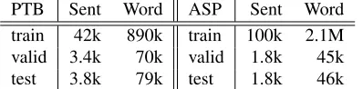
PTB Sent Word ASP Sent Word
train 42k 890k train 100k 2.1M
valid 3.4k 70k valid 1.8k 45k
[image:6.612.328.527.58.107.2]test 3.8k 79k test 1.8k 46k
Table 1: Data sizes for the PTB and ASPEC corpora.
Dst./Ft. HEUR FF LSTM
ML/C 220.5/265.9 146.6/164.5 144.4/162.7
ML/CR - 145.7/163.9 142.6/158.4
KN/C 140.8/156.5 138.9/152.5 136.8/151.1
KN/CR - 136.9/153.0 135.2/149.1
Table 2: PTB/ASPEC perplexities for traditional heuristic (HEUR) and proposed neural net (FF or LSTM) interpolation methods using ML or KN dis-tributions, and count (C) or count+word representa-tion (CR) features.
to post-facto static interpolation of already-trained models (§6.5). For the main experiments, we evalu-ate on two corpora: the Penn Treebank (PTB) data set prepared by Mikolov et al. (2010),3 and the first
100k sentences in the English side of the ASPEC corpus (Nakazawa et al., 2015)4 (details in Tab. 1).
The PTB corpus uses the standard vocabulary of 10k words, and for the ASPEC corpus we use a vocabu-lary of the 20k most frequent words. Our implemen-tation is included as supplementary material.
6.2 Results for Neurally Interpolatedn-grams First, we investigate the utility of neurally interpo-lated n-grams. In all cases, we use a history of N = 5 and test several different settings for the
models:
Estimation type: λ(c)is calculated with heuris-tics (HEUR) or by the proposed method using feed-forward (FF), or LSTM nets.
Distributions:We comparePM L(·)andPKN(·).
For heuristics, we use Witten-Bell for ML and the appropriate discounted probabilities for KN.
Input features: As input features for the neural network, we either use only the count-based features (C) or count-based features together with the word representation for the single previous word (CR).
From the results shown in Tab. 2, we can first see that when comparing models using the same set of
input distributions, the neurally interpolated model outperforms corresponding heuristic methods. We can also see that LSTMs have a slight advantage over FF nets, and models using word representa-tions have a slight advantage over those that use only the count-based features. Overall, the best model achieves a relative perplexity reduction of 4-5% over KN models. Interestingly, even when using simple ML distributions, the best neurally interpo-latedn-gram model nearly matches the heuristic KN method, demonstrating that the proposed model can automatically learn interpolation functions that are nearly as effective as carefully designed heuristics.5
6.3 Results for Neural/n-gram Hybrids
In experiments with hybrid models, we test a neural/n-gram hybrid LM using LSTM networks with both Kronecker δ and KN smoothed 5-gram distributions, trained either with or without block dropout. As our main baseline, we compare to LSTMs with only δ distributions, which have re-ported competitive numbers on the PTB data set (Zaremba et al., 2014).6 We also report results for
heuristically smoothed KN 5-gram models, and the best neurally interpolatedn-grams from the previous section for reference.
The results, shown in Tab. 3, demonstrate that similarly to previous research, LSTM LMs (2) achieve a large improvement in perplexity over n -gram models, and that the proposed neural/n-gram hybrid method (5) further reduces perplexity by 10-11% relative over this strong baseline.
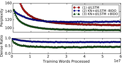
Comparing models without (4) and with (5) the proposed block dropout, we can see that this method contributes significantly to these gains. To examine this more closely, we show the test perplexity for the
5Neurally interpolatedn-grams are also more efficient than standard neural LMs, as mentioned in§4.1. While a standard LSTM LM calculated 1.4kw/s on the PTB data, the neurally in-terpolated models using LSTMs and FF nets calculated 11kw/s and 58kw/s respectively, only slightly inferior to 140kw/s of heuristic KN.
6Note that unlike this work, we opt to condition only on in-sentence context, not inter-sentential dependencies, as training through gradient calculations over sentences is more straight-forward and because examining the effect of cross-boundary information is not central to the proposed method. Thus our baseline numbers are not directly comparable (i.e. have higher perplexity) to previous reported results on this data, but we still feel that the comparison is appropriate.
Dist. Interp. PPL
(1) KN HEUR 140.8/156.5
(2) δ LSTM 105.9/116.9
(3) KN LSTM 135.2/149.1
(4) KN,δ LSTM -BlDO 108.4/130.4
[image:7.612.327.524.57.132.2](5) KN,δ LSTM +BlDO 95.3 /104.5
Table 3: PTB/ASPEC perplexities for traditional KN (1) and LSTM LMs (2), neurally interpolatedn -grams (3), and neural/n-gram hybrid models without (4) and with (5) block dropout.
10 100 1000 Infty
Frequency Cutoff 102
103 104 105
Perplexity
(1) KN/heur (2) d/LSTM (3) KN/LSTM (4) KN+d/LSTM
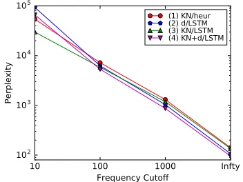
Figure 4: Perplexities of (1) standard n-grams, (2) standard LSTMs, (3) neurally interpolatedn-grams, and (4) neural/n-gram hybrids on lower frequency words.
three models usingδdistributions in Fig. 5, and the amount of the probability mass inλ(c)assigned to
the non-δ distributions in the hybrid models. From this, we can see that the model with block dropout quickly converges to a better result than the LSTM LM, but the model without converges to a worse result, assigning too much probability mass to the dense count-based distributions, demonstrating the learning problems mentioned in§5.2.
It is also of interest to examine exactly why the proposed model is doing better than the more stan-dard methods. One reason can be found in the be-havior with regards to low-frequency words. In Fig. 4, we show perplexities for words that appear n times or less in the training corpus, for n = 10,
[image:7.612.339.515.204.336.2]0 1 2 3 4 5 6 1e7 100
120 140 160
Perplexity
(1) d/LSTM (2) KN+d/LSTM -BlDO (3) KN+d/LSTM +BlDO
0 1 2 3 4 5 6 Training Words Processed 1e7 0.0
0.5 1.0
[image:8.612.79.301.62.172.2]Dense Ratio
Figure 5: Perplexity and dense distribution ratio of the baseline LSTM LM (1), and the hybrid method without (2) and with (3) block dropout.
The neurally interpolated n-gram models consis-tently outperform standard KN-smoothed n-grams, demonstrating their superiority within this model class. In contrast, the neural/n-gram hybrid mod-els tend to follow a pattern more similar to that of LSTM language models, similarly with consistently higher performance.
6.4 Results for Larger Data Sets
To examine the ability of the hybrid models to use counts trained over larger amounts of data, we per-form experiments using two larger data sets:
WSJ: The PTB uses data from the 1989 Wall Street Journal, so we add the remaining years be-tween 1987 and 1994 (1.81M sents., 38.6M words). GW:News data from the English Gigaword 5th Edition (LDC2011T07, 59M sents., 1.76G words).
We incorporate this data either by training net pa-rameters over the whole large data, or by separately training count-basedn-grams on each of PTB, WSJ, and GW, and learning net parameters on only PTB data. The former has the advantage of training the net on much larger data. The latter has two main ad-vantages: 1) when the smaller data is of a particular domain the mixture weights can be learned to match this in-domain data; 2) distributions can be trained on data such as Google n-grams (LDC2006T13), which containn-gram counts but not full sentences. In the results of Fig. 6, we can first see that the neural/n-gram hybrids significantly outperform the traditional neural LMs in the scenario with larger data as well. Comparing the two methods for in-corporating larger data, we can see that the results are mixed depending on the type and size of the data
0 1 2 3 4 5 6 Training Words Processed 1e7 60
80 100 120 140 160
Perplexity
(1) d/p (2) KN+d/p (3) d/w (4) KN+d/w (5) KN+d/p +wLM (6) d/g (7) KN+d/g (8) KN+d/p +gLM
Figure 6: Models trained on PTB (1,2), PTB+WSJ (3,4,5) or PTB+WSJ+GW (6,7,8) using standard neural LMs (1,3,6), neural/n-gram hybrids trained all data (2,4,7), or hybrids trained on PTB with ad-ditionaln-gram distributions (5,8).
being used. For the WSJ data, training on all data slightly outperforms the method of adding distribu-tions, but when the GW data is added this trend re-verses. This can be explained by the fact that the GW data differs from the PTB test data, and thus the effect of choosing domain-specific interpolation coefficients was more prominent.
6.5 Comparison with Static Interpolation
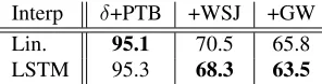
Finally, because the proposed neural/n-gram hybrid models combine the advantages of neural and n -gram models, we compare with the more standard method of training models independently and com-bining them with static interpolation weights tuned on the validation set using the EM algorithm. Tab. 4 shows perplexities for combinations of a standard neural model (orδdistributions) trained on PTB, and count based distributions trained on PTB, WSJ, and GW are added one-by-one using the standard static and proposed LSTM interpolation methods. From the results, we can see that when only PTB data is used, the methods have similar results, but with the more diverse data sets the proposed method edges out its static counterpart.7
[image:8.612.318.534.62.181.2]Interp δ+PTB +WSJ +GW
Lin. 95.1 70.5 65.8
[image:9.612.109.257.57.96.2]LSTM 95.3 68.3 63.5
Table 4: PTB perplexity for interpolation between neural (δ) LMs and count-based models.
7 Related Work
A number of alternative methods focus on interpo-lating LMs of multiple varieties such as in-domain and out-of-domain LMs (Bulyko et al., 2003; Bac-chiani et al., 2006; G¨ulc¸ehre et al., 2015). Perhaps most relevant is Hsu (2007)’s work on learning to interpolate multiple LMs using log-linear models. This differs from our work in that it learns functions to estimate the fallback probabilitiesαn(c)in Eq. 3
instead ofλ(c), and does not cover interpolation of
n-gram components, non-linearities, or the connec-tion with neural network LMs. Also conceptually similar is work on adaptation ofn-gram LMs, which start with n-gram probabilities (Della Pietra et al., 1992; Kneser and Steinbiss, 1993; Rosenfeld, 1996; Iyer and Ostendorf, 1999) and adapt them based on the distribution of the current document, albeit in a linear model. There has also been work incorpo-rating binaryn-gram features into neural language models, which allows for more direct learning ofn -gram weights (Mikolov et al., 2011), but does not af-ford many of the advantages of the proposed model such as the incorporation of count-based probability estimates. Finally, recent works have comparedn -gram and neural models, finding that neural models often perform better in perplexity, butn-grams have their own advantages such as effectiveness in extrin-sic tasks (Baltescu and Blunsom, 2015) and better modeling of rare words (Chen et al., 2015).
8 Conclusion and Future Work
In this paper, we proposed a framework for lan-guage modeling that generalizes both neural net-work and count-based n-gram LMs. This allowed us to learn more effective interpolation functions for count-basedn-grams, and to create neural LMs that incorporate information from count-based models.
As the framework discussed here is general, it is also possible that they could be used in other tasks that perform sequential prediction of words such as
neural machine translation (Sutskever et al., 2014) or dialog response generation (Sordoni et al., 2015). In addition, given the positive results using block dropout for hybrid models, we plan to develop more effective learning methods for mixtures of sparse and dense distributions.
Acknowledgements
We thank Kevin Duh, Austin Matthews, Shinji Watanabe, and anonymous reviewers for valuable comments on earlier drafts. This work was sup-ported in part by JSPS KAKENHI Grant Number 16H05873, and the Program for Advancing Strate-gic International Networks to Accelerate the Circu-lation of Talented Researchers.
References
Waleed Ammar, George Mulcaire, Miguel Ballesteros, Chris Dyer, and Noah A. Smith. 2016. One parser, many languages. CoRR, abs/1602.01595.
Michael Auli and Jianfeng Gao. 2014. Decoder inte-gration and expected bleu training for recurrent neural network language models. InProc. ACL, pages 136– 142.
Michiel Bacchiani, Michael Riley, Brian Roark, and Richard Sproat. 2006. Map adaptation of stochas-tic grammars. Computer Speech and Language, 20(1):41–68.
Paul Baltescu and Phil Blunsom. 2015. Pragmatic neural language modelling in machine translation. InProc.
NAACL, pages 820–829.
Yoshua Bengio, Holger Schwenk, Jean-S´ebastien Sen´ecal, Fr´ederic Morin, and Jean-Luc Gauvain. 2006. Neural probabilistic language models. In
Innovations in Machine Learning, volume 194, pages
137–186.
Thorsten Brants, Ashok C. Popat, Peng Xu, Franz J. Och, and Jeffrey Dean. 2007. Large language models in machine translation. In Proc. EMNLP, pages 858– 867.
Ivan Bulyko, Mari Ostendorf, and Andreas Stolcke. 2003. Getting more mileage from web text sources for conversational speech language modeling using class-dependent mixtures. InProc. HLT, pages 7–9. Stanley F. Chen and Joshua Goodman. 1996. An
empir-ical study of smoothing techniques for language mod-eling. InProc. ACL, pages 310–318.
W. Chen, D. Grangier, and M. Auli. 2015. Strategies for Training Large Vocabulary Neural Language Models.
Stephen Della Pietra, Vincent Della Pietra, Robert L Mer-cer, and Salim Roukos. 1992. Adaptive language modeling using minimum discriminant estimation. In
Proc. ACL, pages 103–106.
Greg Durrett and Dan Klein. 2011. An empirical investi-gation of discounting in cross-domain language mod-els. InProc. ACL.
Irving J Good. 1953. The population frequencies of species and the estimation of population parameters.
Biometrika, 40(3-4):237–264.
C¸aglar G¨ulc¸ehre, Orhan Firat, Kelvin Xu, Kyunghyun Cho, Lo¨ıc Barrault, Huei-Chi Lin, Fethi Bougares, Holger Schwenk, and Yoshua Bengio. 2015. On us-ing monolus-ingual corpora in neural machine translation.
CoRR, abs/1503.03535.
Sepp Hochreiter and J¨urgen Schmidhuber. 1997. Long short-term memory. Neural computation, 9(8):1735– 1780.
Bo-June Hsu. 2007. Generalized linear interpolation of language models. InProc. ASRU, pages 136–140. Rukmini M Iyer and Mari Ostendorf. 1999. Modeling
long distance dependence in language: Topic mixtures versus dynamic cache models. Speech and Audio Pro-cessing, IEEE Transactions on, 7(1):30–39.
Frederick Jelinek and Robert Mercer. 1980. Interpolated estimation of markov source parameters from sparse data. InWorkshop on pattern recognition in practice. Slava M Katz. 1987. Estimation of probabilities from
sparse data for the language model component of a speech recognizer. IEEE Transactions on Acoustics,
Speech and Signal Processing, 35(3):400–401.
Diederik Kingma and Jimmy Ba. 2015. Adam: A method for stochastic optimization.Proc. ICLR. Reinhard Kneser and Hermann Ney. 1995. Improved
backing-off for m-gram language modeling. InProc.
ICASSP, volume 1, pages 181–184. IEEE.
Reinhard Kneser and Volker Steinbiss. 1993. On the dynamic adaptation of stochastic language models. In
Proc. ICASSP, pages 586–589.
Jiwei Li, Michel Galley, Chris Brockett, Jianfeng Gao, and Bill Dolan. 2015. A diversity-promoting objec-tive function for neural conversation models. CoRR, abs/1510.03055.
Tomas Mikolov, Martin Karafi´at, Lukas Burget, Jan Cer-nock`y, and Sanjeev Khudanpur. 2010. Recurrent neu-ral network based language model. In Proc.
Inter-Speech, pages 1045–1048.
Tom´aˇs Mikolov, Anoop Deoras, Daniel Povey, Luk´aˇs Burget, and Jan ˇCernock`y. 2011. Strategies for train-ing large scale neural network language models. In
Proc. ASRU, pages 196–201. IEEE.
Masami Nakamura, Katsuteru Maruyama, Takeshi Kawabata, and Kiyohiro Shikano. 1990. Neural net-work approach to word category prediction for English texts. InProc. COLING.
Toshiaki Nakazawa, Hideya Mino, Isao Goto, Graham Neubig, Sadao Kurohashi, and Eiichiro Sumita. 2015. Overview of the 2nd Workshop on Asian Translation. InProc. WAT.
Hermann Ney, Ute Essen, and Reinhard Kneser. 1994. On structuring probabilistic dependences in stochastic language modelling. Computer Speech and Language, 8(1):1–38.
Vu Pham, Th´eodore Bluche, Christopher Kermorvant, and J´erˆome Louradour. 2014. Dropout improves re-current neural networks for handwriting recognition.
InProc. ICFHR, pages 285–290.
Ronald Rosenfeld. 1996. A maximum entropy approach to adaptive statistical language modelling. Computer
Speech and Language, 10(3):187–228.
Holger Schwenk. 2007. Continuous space language models. Computer Speech and Language, 21(3):492– 518.
Alessandro Sordoni, Michel Galley, Michael Auli, Chris Brockett, Yangfeng Ji, Margaret Mitchell, Jian-Yun Nie, Jianfeng Gao, and Bill Dolan. 2015. A neu-ral network approach to context-sensitive generation of conversational responses. InProc. NAACL, pages 196–205.
Nitish Srivastava, Geoffrey Hinton, Alex Krizhevsky, Ilya Sutskever, and Ruslan Salakhutdinov. 2014. Dropout: A simple way to prevent neural networks from overfitting. The Journal of Machine Learning
Research, 15(1):1929–1958.
Martin Sundermeyer, Ralf Schl¨uter, and Hermann Ney. 2012. LSTM neural networks for language modeling. InProc. InterSpeech.
Ilya Sutskever, Oriol Vinyals, and Quoc VV Le. 2014. Sequence to sequence learning with neural networks.
InProc. NIPS, pages 3104–3112.
Yee Whye Teh. 2006. A Bayesian interpretation of in-terpolated Kneser-Ney. Technical report, School of Computing, National Univ. of Singapore.
Will Williams, Niranjani Prasad, David Mrva, Tom Ash, and Tony Robinson. 2015. Scaling recurrent neural network language models. InProc. ICASSP.
Ian H. Witten and Timothy C. Bell. 1991. The zero-frequency problem: Estimating the probabilities of novel events in adaptive text compression. IEEE
Transactions on Information Theory, 37(4):1085–
1094.
Wojciech Zaremba, Ilya Sutskever, and Oriol Vinyals. 2014. Recurrent neural network regularization.