Abstract—In this paper, a swarm intelligence technique is
presented for solving the fractional differential equations (FDE) based on the cubic spline function and cuckoo search algorithm. In this technique, we approximate FDE with the cubic spline approximation and use the cuckoo search algorithm as a tool for the accurate and rapid solution. Based on this method, the given problem is transformed into a problem for solving a nonlinear equation system, and by solving this system, we obtain the solution of FDE. Furthermore, special attention is given to the error analysis of this method. The presented scheme is evaluated on two initial value problems of FDE. The numerical simulation results demonstrate that the proposed algorithm has higher accuracy and is feasible and effective in solving initial value problem of FDE.
Index Terms—fractional differential equation, cubic spline
approximation, cuckoo search algorithm
I. INTRODUCTION
ITH the development of science and technology, great breakthroughs have been made in theoretical analysis and numerical algorithm of fractional calculus. Analytical solutions of fractional differential equations are usually represented by some special functions, such as Green function, Mittag-Leffler function, and so on. Up to now, the main methods to solve the analytical solutions of fractional differential equations include Fourier transform, Mellin transform, Laplace transform, etc. However, it is an extremely difficult task to find the analytical solution for general fractional differential equation. Therefore, many researchers tend to use numerical approaches to solve the fractional differential equations in the recent thirty years, including linear multi-step method[1-2], finite difference method[3-4], Adomian decomposition method[5], homotopy perturbation method[6-7], variational iteration method[8-9], artificial neural network method[10], collocation method[11-12] and
Manuscript received March 14, 2019; revised September 16, 2019. This work was supported by the Natural Science Foundation of Guangdong Province under Grant No. 2017A030313280
Xinming Zhang (corresponding author) is with the College of Science of Harbin Institute of Technology(Shenzhen), Shenzhen, Guangdong, 518055 PR China(e-mail: [email protected]).
He Huang is with the Department of Probability and statistics of Harbin Institute of Technology (Shenzhen), Shenzhen, Guangdong,
518055 PR China(e-mail: [email protected]).
Xi Zhang is with the Department of Applied Mathematics of Harbin Institute of Technology (Shenzhen), Shenzhen, Guangdong, 518055 PR China(e-mail:[email protected]).
operation matrix method[13-14], the Legendre wavelet method[15], Chebyshev wavelets method[16], the hybrid Taylor series expansion with MHPM[17] , Stochastic methods[18-20], and so on. However, there is still room for investigation into numerical methods which can improve results in terms of accuracy and reliability, with better convenience, e.g. modern intelligent optimization algorithms. These random search algorithms generally based on biological intelligence or physical phenomena and are not perfect in theory. However, from a practical viewpoint, such algorithms usually do not require the continuity and convexity of the objective function and constraints. Even if there is no analytical expression, it is quite adaptable to the uncertain data in calculation, which can overcome the limitations of traditional methods to some extent.
In this paper, Cuckoo Search (CS) algorithm along with cubic splined approximation is used, for the first time as per our literature survey, to solve fractional differential equation. The CS is a swarm intelligent algorithm developed by Yang and Deb in 2009 that inspired from the nature[21]. Due to its favorable efficiency, CS has been attracting considerable attentions since it was born and has shown promising superiority in many science and engineering fields, such as inverse problems and shape optimization[22], phase equilibrium and stability calculations[23], structural optimization[24], hydraulic parameter estimation problem[25], solution of nonlinear equation system[26], multi-objective optimal power flow[27], hyperspectral image classification[28], and so on. To the best of our knowledge, the application of CS along with cubic splined approximation (CS-CS) to solve fractional differential equation has not been reported, and for the first time, this topic is investigated in the literature. The aim of our study is to identify the relative strengths of the proposed algorithm for the solution of fractional differential equation. This study shows that CS-CS algorithm offers a reliable performance for solving these differential equation of fractional order.
The rest of this paper is organized as follows: In Section 2 some basic definitions and the proposed numerical algorithm (CS-CS) are given. Section 3 shows the error analysis of the presented method. In Section 4, several numerical experiments are conducted to verify the feasibility and effectiveness of the proposed method for solving fractional differential equations, and finally, the conclusions are derived in Section 5.
Xinming Zhang, He Huang, and Xi Zhang
Applying Cuckoo Search Algorithm to Solve
Fractional Differential Equation Based on Cubic
Spline Function
W
IAENG International Journal of Applied Mathematics, 50:1, IJAM_50_1_05
II. MATHEMATICAL MODEL FOR SOLVING FRDE For positive real number v , 0 n 1 v n , the order v Caputo fractional derivative of the function f t( ) defined on the interval [0, ]T is
1 0 1, 0 1 ,
, . n t v n C v a t n n f d
if n v n
n v t
D f t d
f t if v n N
dt
(1)The generic non-linear quadratic fractional differential equations solved in this article can be written as
2 ( )
( ) ( ) ( ) ( ) ( ), 0 v
v
d y t
p t q t y t r t y t t T dt
(2)
with initial condition given as
(0)
,
0,1, 2,...,
1
k
k k
d
y
c k
n
dt
, (3)where vis the order which satisfies v0, v , n v .
( )
y t is the solution of the fractional differential equation.
( ), ( ), ( )
p t q t r t are known functions, and T c, k are known
parameters.
A. Cubic spline approximation
For the initial value problem of fractional differential equation (2) and (3), in this sub-section, we discretize fractional differential equations into nonlinear algebraic equations by cubic spline function.
Taking m1 nodes on the interval [0, ]T and dividing the interval intomsubintervals [ , ],[ , ],...,[ ,t t1 2 t t2 3 tm tm 1 ].Using a cubic spline function on each subinterval, that is
3 2
1
( )
,
,
1, 2,..., .
i i i i i i i
y t
a t
b t
c t
d t
t
t
i
m
(4) Since the second derivative of the cubic spline is continuous, we have1 1 1
ˆ
( )
ˆ
( )
,
1, 2,...,
1
i i
i t t i t t
y t
y
t
i
m
1 1
(1) (1)
1
ˆ
( )
ˆ
( )
,
1, 2,...,
1
i i
i t t i t t
y
t
y
t
i
m
1 1
(2) (2)
1
ˆ
( )
ˆ
( )
,
1, 2,...,
1
i i
i t t i t t
y
t
y
t
i
m
Since the above equations satisfy the initial condition
0
ˆ(0)
y
y
, we can getat
3
bt
2
ct
d
t0
y
0 , that is 0d
y
.Then take l small nodes on each subinterval, and let the function value of each small node approximate the fractional differential equation. So there is
2 ( )
( )
( ) ( )
i( )
i( )
iv( ) ,
1, 2,...,
.
p t
q t y t
r t y
t
y
t
i
m l
(5)Thus, the problem is transformed into the following nonlinear algebraic equations with undetermined coefficients. 1) Case 1.
0
v
1
,1 1 1 1 1 1 1 1 1 1 0 2
ˆ
( )
ˆ
( )
,
1, 2,...,
1
ˆ
( )
ˆ
( )
,
1, 2,...,
1
ˆ
( )
ˆ
( )
,
1, 2,...,
1
ˆ
( )
( )
( ) ( )
ˆ
( )
ˆ
( ),
1, 2,...,
i i
i i
i i
i t t i t t
i t t i t t
i t t i t t
v i
y t
y
t
i
m
y t
y
t
i
m
y t
y
t
i
m
d
y
y t
p t
q t y t
r t y t
i
m l
(6) where t( ) 2
0 2 0 0 0 2 1 0 1 1 0 1
ˆ ( ) ( ) (3 2 )d
(1 ) 3
( ) d (1 )
2
( ) d ( ) d
(1 ) (1 )
3
d( ) (1 ) (1 )
2
d( ) (1 ) (1 ) (1 ) (1 )
6 (1 ) (1
v v
i i i i
t v i t t v v i i t v i t v v i i i
y t t a b c
v a t v c b t t v v a t v v c b t t
v v v v
a v
1 0 1 2 3 1 2( ) d )
2
(1 ) (1 ) (2 )(1 ) (1 ) 6
(3 )(2 )(1 ) (1 ) 2
. (1 ) (1 ) (2 )(1 ) (1 )
t v v v i i v i v v i i t v c b t t
v v v v v
a
t
v v v v
c b
t t
v v v v v
(7) 2) Case 2.1
v
2
,1 1 1 1 1 1 1 1 1 1 0 1 0 2
ˆ
( )
ˆ
( )
,
1, 2,...,
1
ˆ
( )
ˆ
( )
,
1, 2,...,
1
ˆ
( )
ˆ
( )
,
1, 2,...,
1
ˆ
( )
( )
( ) ( )
ˆ
( )
ˆ
( ),
1, 2,...,
.
i i
i i
i i
i t t i t t
i t t i t t
i t t i t t
v i
y t
y
t
i
m
y t
y
t
i
m
y t
y
t
i
m
d
y
c
y
y t
p t
q t y t
r t y t
i
m l
(8) where 1 t ( ) 0 1 1 0 0 2 2 2 0 0 2 3 1ˆ ( ) ( ) (6 2 )d (2 )
2 6
( ) d ( ) d
(2 ) (2 )
2 (2 ) (2 )
6
( ) ( ) d
(2 ) (2 )
2 6
. (2 ) (2 ) (3 )(2 ) (2 )
v v
i i i
v v t t i i v i v t v t i v v i i
y t t a b
v b a t t v v b t v v a t t v v b a t t
v v v v v
(9)IAENG International Journal of Applied Mathematics, 50:1, IJAM_50_1_05
3) Case 3.
2
v
3
,1 1
1 1
1 1
1 1 1 1 0
1 0 1 0
2
ˆ
( )
ˆ
( )
,
1, 2,...,
1
ˆ
( )
ˆ
( )
,
1, 2,...,
1
ˆ
( )
ˆ
( )
,
1, 2,...,
1
2
ˆ
( )
( )
( ) ( )
ˆ
( )
ˆ
( ),
1, 2,...,
.
i i
i i
i i
i t t i t t
i t t i t t
i t t i t t
v i
y t
y
t
i
m
y t
y
t
i
m
y t
y
t
i
m
d
y
c
y
b
y
y t
p t
q t y t
r t y t
i
m l
(10)where
2 ( )
0
3 0
3
3
1
ˆ ( ) ( ) 6 d (3 )
6 1
( ) (3 ) 3
6 1
0
(3 ) 3
6 1
. (3 ) 3
v t v
i i
v t i
v i
v i
y t t a
v a
t
v v
a
t
v v
a
t
v v
(11)
To sum up, transforming the initial value problem of fractional differential equation into a nonlinear equation model involves three steps. First, we divide the interval
[0, ]T into m subintervals , [ , ],[ , ],...,[ ,t t1 2 t t2 3 tm tm 1], and
express the unknown function with cubic spline
function in each interval
3 2
ˆ ( )
i i i i iy t
a t
b t
c t
d
,t
i
t
t
i1 i1, 2, ...,m.Seco nd, based on the fact that the second derivative of cubic spline function is continuous, we transform the fractional differential equation into a model of nonlinear equations. Third, for the party
ˆ ( )
i( )vt
which is difficult to solve in the nonlinear equations model, we discuss it in several cases.B. Implementation of cuckoo search algorithm
After transforming the fractional differential equation into a nonlinear equations model, common traditional algorithms for solving nonlinear algebraic equations include newton method, conjugate gradient method, least squares method, etc. However, it has been pointed out that these methods require extremely high in the selection of initial points. In recent years, several modern intelligent algorithms have been developed to calculate nonlinear equations, such as Genetic algorithm, particle swarm algorithm, ant colony algorithm, etc. These algorithms not only overcome the problem of selecting the initial points existing in traditional algorithms, but also have strong global optimization ability to some extent. In this section, we will use the cuckoo search algorithm to solve the transformed nonlinear equations. In order to better implement the cuckoo search algorithm, three ideal states are assumed:
(1) Each cuckoo produces only one egg at a time, and randomly chooses a nest to place it;
(2) In the process of searching bird's nest, we calculate the optimal nest position and save it to the next generation;
(3) The probability of host finding cuckoo’s eggs and abandoning them is
p p
a,
a
[0,1]
.Thus, the update formula of cuckoo search can be
expressed as
( 1) ( )
( ),
1, 2, 3,...,
t t
i i
x
x
L
i
n
, (12)where
x
i( )t indicates the position of thei
th bird nest in thet
th iteration;
represents the step size, usually take
1
;
L obeys Levy distribution
( ) 1
( )
0.01
(
t t), 0
2,
j i
u
L
x
x
v
(13),
u v obeys normal distribution,
2
2
~ 0, u , ~ 0, v
u N
v N
,
1 1 2
1
sin
2
1
2
2
1.
u
v
(14)
In this way, we can refer to the cuckoo search for the optimal nest and hatching process to implement the cuckoo search algorithm. The specific steps are as follows:
Step 1: Define and initialize the objective function ( ), ( ,1 2,..., )T
d
f X X x x x ,d is the dimension of bird's nest, and randomly generate
n
initial nest position( 1, 2,..., ) i
X i n . Initialize the rejection probability
p
a. Step 2: Calculate the value of objective function of each bird nest position, and select the bird nest with the optimal value.Step 3: Preserve the optimal nest location of the previous generation, and update the nest location with Levy flight (13). Step 4: Compare the current value of position function with the previous optimal value. If better, update the value of the current objective function, otherwise, retain the optimal value of the previous generation.
Step 5: After updating the position, generate the random number
r
[0,1]
. Ifr
p
a, renewx
i(t1)and compare the new nest, then calculate the global positionpb
t*.Step 6: Determine whether
f pb
(
t*)
meets the maximum iterations or minimum error requirement, and if so, the output*
(
t)
f pb
is the global optimal solutiongb
.Otherwise, return to step 2.III. ERROR ANALYSIS
In this section, we will analyze the error of approximating the solution function of the fractional differential equation with cubic spline function, and derive the convergence order. For general nonlinear quadratic fractional differential equation
2
( )
( ) ( ) ( ) ( ) ( ), [0, ] 0,
v
v d y t
p t q t y t r t y t t T v
dt
, (15)
(0) , 0,1, 2, ..., 1,
k
k k
d
y C k n n v
dt , (16)
Taking m1 nodes on the interval [0, ]T and dividing the interval into m subintervals, [ , ],[ , ],...,[ ,t t1 2 t t2 3 tm tm 1 ] . Using a cubic spline function on each subinterval, one gets
3 2
1
( ) , ,
1, 2,..., .
i i i i i i
i
y t a t b t c t d t t t
i m
(17)
IAENG International Journal of Applied Mathematics, 50:1, IJAM_50_1_05
and
2
ˆ
( )
3
2
,
ˆ
( )
ˆ
6
2 ,
( )
6
i i i i i
i i i i
y t
a t
b t
c y
t
a t
b y
t
a
(18)Using Taylor expansion on the interval [ ,t ti i1], we have
3 2
3 2
2
2 3 3
2
3 3
ˆ ( )
(3 2 )( )
(6 2 ) 6
( ) ( ) ( )
2! 3!
ˆ ( )
ˆ( ) ˆ( )( ) ( )
2! ˆ ( )
( ) ( ),
3!
i i i i i
i i i i i i i
i i i i i i
i i i i
i i
i i
i i i i i i
i i i
y t a t b t c t d a t b t c t d
a t b t c t t
a t b a
t t t t o h
y t y t y t t t t t
y t
t t o h
(19) 2 2 2 2
ˆ ( ) 3 2
3 2 (6 2 )( )
6
( ) ( ),
2!
i i i i
i i i i i i i i i
i i
y t a t b t c
a t b t c a t b t t a
t t o h
(20)
ˆ ( ) 6 2
6 2 6 ( ) ( ).
i i i
i i i i i
y t a t b
a t b a t t o h
(21)
The real analytic solution y ti( ) of (15) and (16) can be
expanded to 2 3 ( ) ( ) ( ) ( )( ) ( ) 2! ( ) ( ) ( ) ... ( ) ( ) 3! ! i i
i i i i i i i
n
n n
i i i i
i i
y t
y t y t y t t t t t
y t y t
t t t t o h
n 2 ( ) 1 1
( )
( )
( )
( )(
)
(
)
2!
( )
...
(
)
(
)
(
1)!
i ii i i i i i i
n
n n
i i
i
y
t
y t
y t
y
t
t
t
t
t
y
t
t
t
o h
n
( ) 2 2( )
( )
( )(
)
( )
...
(
)
(
)
(
2)!
i i i i i i
n
n n
i i
i
y
t
y
t
y
t
t
t
y
t
t
t
o h
n
Then, we get
2 3 3
(4) ( )
4
( ) ( )
( ) ( ) ( ( ) ( ))( )
( ) ( ) ( ) ( )
( )( ) ( )( ) ( )
2! 2! 3! 3!
( ) ( )
( ) ... ( ) ( )
4! !
i i
i i i i i i i i i
i i i i i i i i
i i
n
n n
i i i i
i i
y t y t
y t y t y t y t t t
y t y t y t y t
t t t t o h
y t y t
t t t t o h
n 2 2
(4) ( )
3 1 1
( ) ( ) ( ) ( ) ( ( ) ( ))( ) ( ) ( ) ( )( ) ( ) 2! 2! ( ) ( ) ( ) ... ( ) ( )
3! ( 1)!
i i
i i i i i i i i i
i i i i
i
n
n n
i i i i
i i
y t y t
y t y t y t y t t t y t y t
t t o h
y t y t
t t t t o h
n (4) (5) 2 3 ( ) 2 2 ( ) ( ) ( ) ( ) ( ( ) ( ))( ) ( ) ( ) ( ) ( ) ( ) 2! 3! ( ) ... ( ) ( ) ( 2)! i i
i i i i i i i i i
i i i i
i i
n
n n
i i i
y t y t
y t y t y t y t t t o h
y t y t
t t t t
y t
t t o h n
According to (10), fractional differential equation (15) and (16) can be reduced to the following equations
1 1 1 1 1 1 1 1 1
1 0 1
1 0 2
1 0 3
2
( ) ( ) , 1, 2,..., 1
( ) ( ) , 1, 2,..., 1
( ) ( ) , 1, 2,..., 1
2 ( ) ( ) ( ) ( ) ( ) ( ), 1, 2,..., i i i i i i
i t t i t t
i t t i t t
i t t i t t
v i
y t y t i m
y t y t i m
y t y t i m
d y C
c y C
b y C
y t p t q t y t r t y t
i m l
(22) Theorem 1
If the analytical solution y t( )of the problem (15) and (16) has n order continuous derivative on the interval [0, ]T , then the local truncation error of the approximate solution function
ˆ ( ),i 1, 2,...
y t i mused to simulate the real analytic solution
( )
y t is o h( 3) . Proof:
On the interval [ , ]t t1 2 , where t10 ,
1 1
1 1 1 1 1 1 1 1 1
2 3
1 1 1
1 1
1
(4) ( )
3 1 4 1 1
1 1
3 1
1 1 2 1
( )
( )
( )
( ) (
( )
( ))(
)
( )
( )
( )
( )
(
)(
)
(
)(
)
2!
2!
3!
3!
( )
( )
(
)
(
)
...
(
)
(
)
4!
!
2
(
)
(
)
2!
2!
i i i
i
n
n n
i
y t
y t
y t
y t
y t
y t
t
t
y
t
y
t
y
t
y
t
t
t
t
t
y
t
y
t
o h
t
t
t
t
o h
n
C
b
C
d
C
c t
2 1 1 3(4) ( )
3 1 4 1
3 3
1 1
(4) ( )
4 1 1 3 1 1
(0)
6
(
)
3!
3!
(0)
(0)
(
)
...
(
)
4!
!
(0)
6
= (
)
(
)
3!
3!
(0)
(0)
...
(
)
4!
!
(0)
6
1
(
)
3!
3!
n n n n n ny
a
t
t
y
y
o h
t
t
o h
n
y
a
t
o h
y
y
t
t
o h
n
y
a
o h
IAENG International Journal of Applied Mathematics, 50:1, IJAM_50_1_05
1 1
1 1 1 1 1 1 1 1 1
2 2
1 1 1 1 1
(4) ( )
3 1 1
1 1 1 1
1 1
2
1 1
2 1 3 1
2 ( ) ( ) ( ) ( ) ( ( ) ( ))( ) ( ) ( ) ( )( ) ( ) 2! 2! ( ) ( ) ( ) ... ( ) ( )
3! ( 1)!
(0) 6
( 2 ) ( )
2! 2!
( )
n
n n
y t y t
y t y t y t y t t t y t y t
t t o h
y t y t
t t t t o h
n
y a
C c C b t t
o h
1(4) 3 1( ) 1 1
2 2
1 1
(4) ( )
3 1 1
1 1
2
1 1
(0) (0)
... ( )
3! ( 1)!
(0) 6
( ) ( )
2! 2!
(0) (0)
... ( )
3! ( 1)!
(0) 6
1 ( )
2! 2! n n n n n n y y
t t o h
n
y a
t o h
y y
t t o h
n y a o h 1 1
1 1 1 1 1 1 1 1 1
(4) (5)
2 3
1 1 1 1
1
( )
2 2
1 1
1
2 1 1 1 1
(4) (5) 2 1 1 ( ) ( ) ( ) ( ) ( ( ) ( ))( ) ( ) ( ) ( ) ( ) ( ) 2! 3! ( ) ... ( ) ( ) ( 2)!
2 ( ( ) 6 ) ( )
(0) (0)
2! 3!
i
n
n n
y t y t
y t y t y t y t t t o h
y t y t
t t t t
y t
t t o h n
C b y t a t o h
y y t
3 1( ) 2 2
1 1
(0)
... ( )
( 2)!
(0) 6 1 ( )
n
n n
y
t t o h
n
y a o h
On the interval [ , ]t t2 3 ,
2 2
2 2 2 2 2 2 2 2 2
2 3 3
2 2 2 2 2 2 2 2
2 2
(4) ( )
4
2 2 2 2
2 2
1 2 1 2 1 2
ˆ ( ) ( ) ˆ ˆ ( ) ( ) ( ( ) ( ))( ) ˆ ˆ ( ) ( ) ( ) ( ) ( )( ) ( )( ) ( )
2! 2! 3! 3!
ˆ ( ) ˆ ( )
( ) ... ( ) ( ) 4! ! ˆ ˆ ( ) ( ) ( ) n n n
y t y t
y t y t y t y t t t
y t y t y t y t
t t t t o h
y t y t
t t t t o h
n y t y t y t
1 2
2 3 3
1 2 1 2 2 2 2 2
2
(4) ( )
4
2 2 2 2
2 2
( ) ( )
ˆ ˆ
( ) ( ) ( ) ( )
( ) ( )( ) ( )
2! 2! 3! 3!
ˆ ( ) ˆ ( )
( ) ... ( ) ( )
4! !
n
n n
y t o h
y t y t y t y t
o h t t o h
y t y t
t t t t o h
n 3 2
1 1 1 1
2 2 2 2 2 3
1 1
(4) ( )
4
2 2 2 2
2 2
1 1 1
(0) 6 (0) 6
1 ( ) 1 ( ) ( )
3! 3! 2! 2!
ˆ ( ) ( ) 1
(0) 6 1 ( ) ( ) 1 ( )
2! 3! 3!
ˆ ( ) ˆ ( )
( ) ... ( ) ( )
4! !
(0) 6 (0) 6 1
3! 3! 2!
n
n n
y a y a
o h o h o h
y t y t
y a o h o h o h
y t y t
t t t t o h
n
y a y
1
3
2 2 2 2
1 1 1 2! ˆ ( ) ( ) 1
(0) 6 1 1 ( ).
2! 3! 3!
a
y t y t
y a o h
In the same way, on each interval
1 2 2 3 1
[ , ],[ , ],...,[ ,t t t t tm tm ], we have
3
( )
( )
(
)
i i i
y t
y t
C
o h
where Ci is an appropriate positive constant,i1, 2, ...,m. IV. NUMERICAL EXAMPLES
In order to verify the feasibility and effectiveness of the new proposed method for solving fractional differential equations. In this section, we will present two numerical experiments based on the previous discussion.
A. Example 1
Consider fractional differential equation
2 2
( ) 2
( ), 0, (0) 0, 0 1. (3 )
v
v v
d y t
t t y t t y v
v dt ( 23)
The exact solution of this equation is
2
( )
.
y t
t
According to (6), (23) can be transformed into the following equations: 1 1 1 1 1 1 1 1 1 1 (2) (2) 1 1
2 2 1
2
( ) ( ) , 1, 2,... 1
( ) ( ) , 1, 2,... 1
( ) ( ) , 1, 2,... 1
0 2
0 ( )
(3 ) (1 ) (1 )
2 6
(2 )(1 ) (1 ) (3
i i
i i
i i
i t t i t t
i t t i t t
i t t i t t
v i v
i
v
i i
y t y t i m
y t y t i m
y t y t i m
d
c
t t y t t
v v v
b a
t
v v v
( ) ( ) 3 , )(2 )(1 ) (1 ) 1, 2,...,
v
t
v v v v
i m l
For convenience, we first select
0.5, 1, 20, 1
v m l T . At this time, the error tolerance can reach Tol1015 , which takes 12.313966 seconds.
Moreover, in order to increase the credibility of the numerical simulation, the results are averaged by considering 30 different executions. The comparison results are shown in Fig.1. As we can see that the solution obtained by CS-CS is almost close to the real analytical solution. Table I lists the numerical solution and the error comparison of these methods. From Table I, we can find that the accuracy of the cuckoo search algorithm based on cubic spline approximation (CS-CS) is much higher than the particle swarm optimization based on artificial neural network (PSO-ANN) and
GrunwaldLetnikov classical numerical method[19].
IAENG International Journal of Applied Mathematics, 50:1, IJAM_50_1_05
TABLEI
PSO-ANN,GL,CS-CSCOMPARISON TABLE AT t=[0,1]
t Exact
solution
Solution of GL
Solution of PSO-ANN
Solution of CS-CS
Error by GL
Error by PSO-ANN
Error by CS-CS
0.0 0.00000 0.00000 5.45e-6 0.00000000000000 0 5.45e-6 5.2e-18
0.2 0.04000 0.04007 0.04045 0.04000000000000 7e-5 4.52e-4 0
0.3 0.09000 0.09011 0.09072 0.09000000000000 1.1e-4 7.18e-4 0
0.4 0.16000 0.16013 0.16045 0.16000000000000 1.3e-4 4.51e-4 0
0.5 0.25000 0.25016 0.24958 0.25000000000000 1.6e-4 4.25e-4 0
0.6 0.36000 0.36019 0.35827 0.36000000000000 1.9e-4 1.73e-3 -5.551e-17
0.7 0.49000 0.49021 0.48693 0.49000000000000 2.1e-4 3.07e-3 -5.551e-17
0.8 0.64000 0.64023 0.63619 0.64000000000000 2.3e-4 3.81e-3 0
0.9 0.81000 0.81026 0.80688 0.81000000000000 2.6e-4 3.11e-3 0
1.0 1.00000 1.00028 1.00004 1.00000000000000 2.8e-4 4.40e-5 0
Fig. 1. Comparison of PSO-ANN, GL, CS-CS at t = [0, 1] Fig. 2. Simulation diagram of by CS-CS at t = [0, 2]
Fig. 3. Simulation diagram of by CS-CS at t = [0, 10] Fig.4. Simulation diagram of by CS-CS at t = [0, 100] CS-CS
Exact
GL
PSO-ANN
IAENG International Journal of Applied Mathematics, 50:1, IJAM_50_1_05
[image:6.595.48.566.280.760.2]TABLE II
COMPARISON OF RESULTS FOR THE SOLUTION OF EXAMPLE 1(v =0.25,t =[0,1])
t Exact solution Error by EOC Error by FWCW Mean error by CS-CS
0.09375 0.0087890625 1.15137021309e-5 0.43017672757 e-13 1.243218491116710e-17
0.18750 0.0351562500 1.34008681836e-5 0.53908266740 e-13 1.989149585786740e-17
0.28125 0.0791015625 1.45485346092e-5 0.24466539905 e-13 1.850371707708590e-17
0.37500 0.1406250000 1.53757162245e-5 0.03941291737 e-13 1.757853122323160e-17
0.46875 0.2197265625 1.60223410662e-5 0.64837024638 e-13
2.312964634635740e-17 0.56250 0.3164062500 1.65528139359e-5 0.54012350148 e-13 2.035408878479450e-17
0.65625 0.4306640625 1.70022170524e-5 0.09825473768 e-13 3.515706244646330e-17
0.75000 0.5625000000 1.73918021056e-5 0.17985612999 e-13
1.480297366166880e-17 0.84375 0.7119406250 1.77354280767e-5 0.31863400807 e-13 3.330669073875470e-17
0.93750 0.8789062500 1.80426383865e-5 2.01283434365 e-13 4.810966440042350e-17
TABLE III
COMPARISON OF RESULTS FOR THE SOLUTION OF EXAMPLE 1(v =0.75,t =[0,1])
t Exact solution Error by EOC Error by FWCW Mean error by CS-CS
0.09375 0.0087890625 0.201409844130e-3 0.347308987125e-13 1.295260195396020e-17 0.18750 0.0351562500 0.312234854242e-3 0.022967738822e-13 2.012279232133100e-17 0.28125 0.0791015625 0.397141377633e-3 0.198174809896e-13 2.359223927328460e-17 0.37500 0.1406250000 0.466219134874e-3 0.293931545769e-13 2.683038976177460e-17 0.46875 0.2197265625 0.524234122143e-3 0.221489493413e-13 2.220446049250310e-17 0.56250 0.3164062500 0.573965121404e-3 0.194289029309e-13 2.775557561562890e-17 0.65625 0.4306640625 0.617222689041e-3 0.170974345793e-13 2.775557561562890e-17 0.75000 0.5625000000 0.655271385754e-3 0.091038288019e-13 2.220446049250310e-17 0.84375 0.7119406250 0.689037602412e-3 0.119904086659e-13 4.810966440042350e-17 0.93750 0.8789062500 0.719224088406e-3 0.275335310107e-13 6.661338147750940e-17
Fig.5. Error comparison of EOC,FWCW,CS-CS at v =0.25,t =[0,1] Fig.6. Error comparison of EOC,FWCW,CS-CS at v =0.75,t =[0,1]
In addition, CS-CS not only has high accuracy at interval
[0,1]
t , but also maintains high accuracy and stability
when the range of Tbecomes larger. Fig. 2, 3, 4 are the simulated diagram of numerical solutions obtained by EOC
FWCW
CS-CS
EOC
FWCW
CS-CS
IAENG International Journal of Applied Mathematics, 50:1, IJAM_50_1_05
CS-CS at intervals t[0, 2],t[0,10] andt[0,100], respectively. These three cases take 15.068018 seconds, 17.216479 seconds and 20.749634 seconds, respectively. Even for the case t[0,100] , the accuracy of the numerical solution can be as high as 13
10 , which shows that the algorithm still has high accuracy and stability when the Tvalue keeps increasing.
In order to show the superiority of CS-CS in further, the value of the fractional order derivative ν is taken as 0.25 and 0.75. The corresponding results are summarized in Table II, Table III and Fig.5, Fig.6. It also contains reported results with FWCM[29] and EOC[30]. It can be inferred that our algorithm provides an approximate solution to the fractional differential equation more effectively.
B. Example 2
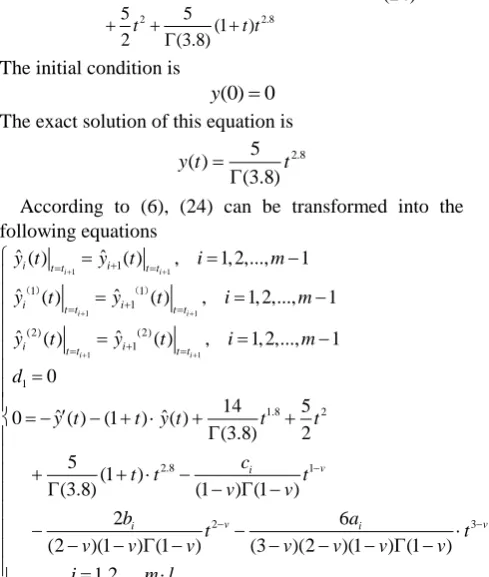
Consider the fractional differential equation
0.8
1.8 0.8
2 2.8
d ( ) 14
( ) (1 ) ( ) (3.8) d
5 5
(1 ) 2 (3.8)
y t
y t t y t t
t
t t t
(24)
The initial condition is
(0) 0
y The exact solution of this equation is
2.8 5 ( )
(3.8)
y t t
According to (6), (24) can be transformed into the following equations
1 1
1 1
1 1
1
1 1
1
(2) (2)
1
1
1.8 2
2.8
ˆ( ) ˆ ( ) , 1, 2,..., 1
ˆ ( ) ˆ ( ) , 1, 2,..., 1
ˆ ( ) ˆ ( ) , 1, 2,..., 1
0
14 5
ˆ ˆ
0 ( ) (1 ) ( )
(3.8) 2
5
(1 )
(3.8) (
i i
i i
i i
i t t i t t
i t t i t t
i t t i t t
i
y t y t i m
y t y t i m
y t y t i m
d
y t t y t t t
c t t
( ) ( )
1
2 3
1 ) (1 )
2 6
,
(2 )(1 ) (1 ) (3 )(2 )(1 ) (1 )
1, 2,..., .
v
v v
i i
t
v v
b a
t t
v v v v v v v
i m l
In the following, we will use cuckoo search algorithm to calculate the above equations and discuss the influence of the parameter
l
.(1)Choose m2,l10,T 1,Tol1.1227 . It takes 16.439011 seconds. The coefficient solutions are:
1 2
1 2
1 2
1 2
0.925561212447776 0.738891012901748 0.179615628191602 0.459623589255583 0.015345206321721 0.155256770376138 0.000000008744638 0.023283177842368,
a a
b b
and
c c
d d
We get the approximate solution of the equation:
3 2
1
3 2
2
ˆ( )
( ) 0.925561212447776 0.179615628191602
0.015345206321721 0.000000008744638 0 0.5 ( ) 0.738891012901748 0.459623589255583
0.155256770376138 0.023283177842368 0
y t
y t t t
t t
y t t t
t
.5 t 1.
(2) Choosem2,l20,T 1,Tol1.1714 . It takes 27.7729821 seconds. The coefficient solutions are:
1 2
1 2
1 2
1 2
0.919498494305771 0.750548643123485 0.183727300560656 0.437107118636707 0.015943443439072 0.142555742170239
0.000000014508539 0.021816521494590,
a a
b b
and
c c
d d
The approximate solution of the equation is:
3 2
1
3 2
2
ˆ( )
( ) 0.919498494305771 0.183727300560656
0.015943443439072 0.000000014508539 0 0.5 ( ) 0.750548643123485 0.437107118636707
0.142555742170239 0.021816521494590 0
y t
y t t t
t t
y t t t
t
.5 t 1.
(3) Choosem2,l30,T 1,Tol1.2156 . It takes 27.7729821 seconds. The coefficient solutions are:
1 2
1 2
1 2
1 2
0.925913752517327 0.754732405733558 0.178866218377388 0.427150121741720 0.015223271257590 0.134842553318408 0.000000025245317 0.019562451330709,
a a
b b
and
c c
d d
This yields:
3 2
1
3 2
2
ˆ( )
( ) 0.925913752517327 0.178866218377388
0.015223271257590 0.000000025245317 0 0.5 ( ) 0.754732405733558 0.427150121741720
0.134842553318408 0.019562451330709 0
y t
y t t t
t t
y t t t
t
.5 t 1.
Table IV lists the error comparison between the numerical solutions obtained by CS-CS and the analytical solution whenl10,l20,andl30. The Mean square error(MSE) of three cases are MSE_l10=2.2772e-5, MSE_l20=1.7102e-5, MSE_l30=2.1554e-5, respectively. We can find that the error is relatively small at around 105
forl20.
Fig.7 shows the numerical solutions obtained with CS-CS (l20) and difference method(DM) in [31].From Fig.7,we can observe that the solution obtained by CS-CS is closer to analytical solution than DM. In addition, Table V lists the error comparison between the exact solutions and numerical solutions by CS-CS and DM methods at several points. It is shown that the numerical solution accuracy of CS-CS is around104 ~ 105, which is more
close to the real analytical solution than DM method. Table VI lists the maximum error, the minimum error and the mean error of CS-CS for 30 experiments.
IAENG International Journal of Applied Mathematics, 50:1, IJAM_50_1_05
[image:8.595.315.552.57.421.2] [image:8.595.47.292.304.593.2]Fig.7. Comparison of CS-CS,DM at t=[0,1],v=0.8
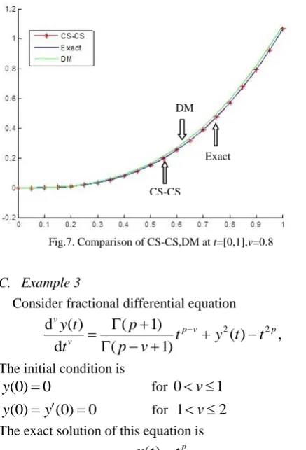
C. Example 3
Consider fractional differential equation
2 2
d
( )
(
1)
( )
,
d
(
1)
v
p v p
v
y t
p
t
y t
t
t
p
v
(25)The initial condition is
(0)
0
y
for0
v
1
(0)
(0)
0
y
y
for 1
v
2
The exact solution of this equation is( )
py t
t
In the following, we will discuss the solution of (25) in different cases.
Case 1. p3,v0.5
According to (7), (25) can be transformed into the following equations
1 1
1 1
1 1
1
(1) (1)
1
(2) (2)
1
1
2 2 1
ˆ( ) ˆ ( ) , 1, 2,..., 1
ˆ ( ) ˆ ( ) , 1, 2,..., 1
ˆ ( ) ˆ ( ) , 1, 2,..., 1
0 (4)
0 ( )
(4 ) (1 ) (1 )
2
(2 )(1 ) (
i i
i i
i i
i t t i t t
i t t i t t
i t t i t t
p v p i v
i
i
y t y t i m
y t y t i m
y t y t i m
d
c
t y t t t
v v v
b
v v
2 6 3
,
1 ) (3 )(2 )(1 ) (1 )
1, 2,..., .
v ai v
t t
v v v v v
i m l
The parameter is chosen as
1 1, 10, 0.4182
m ,T l Tol .Using cuckoo algorithm to calculate the above equations, and it takes 4.8807
[image:9.595.320.551.106.427.2]seconds. The simulation results are shown in Fig.8 and Table VII. As we can see that the numerical solution agree well with the analytical solution and the mean error of CS-CS can reach 10-7.
2) Case 2. p3,v1.5
According to (9), (25) can be transformed into the following equations
1 1
1 1
1 1
1
(1) (1)
1
(2) (2)
1 1
1
2
3
ˆ ( ) ˆ ( ) , 1, 2, , 1
ˆ ( ) ˆ ( ) , 1, 2, , 1
ˆ ( ) ˆ ( ) , 1, 2, , 1
0 0
(4) 2
0
(4 ) (2 ) (2 )
6 ˆ
(3 )(2 ) (1 )
i i
i i
i i
i t t i t t
i t t i t t
i t t i t t
p v i v
v i
i
y t y t i m
y t y t i m
y t y t i m
d c
b
t t
v v v
a
t y
v v v
2 2
( ) ,
1, 2, , 1.
p
t t
i m
Similarly, the parameter is chosen asm1,T1,l10,Tol1015. It takes 10.7952 seconds for cuckoo algorithm to calculate the above equations. Fig.9 and Table VIII give the simulation results. We can conclude that the numerical solution are found in well agreement with the analytical solution and the mean error of CS-CS can reach10-16.
V. CONCLUSION
In this paper, we propose a new solution scheme for the initial value problem of fractional differential equations, which is solved by cuckoo search algorithm based on cubic spline (CS-CS). A cubic spline function was introduced to transform the fractional differential equations into nonlinear equations and the Cuckoo search algorithm was applied to solve the nonlinear equation system. Furthermore, we derive the convergence order which proves the theoretical feasibility of the proposed method. By using CS-CS algorithm to solve specific examples, we find that the new method has the characteristics of high precision and fast convergence speed. Therefore, the cuckoo algorithm based on cubic spline (CS-CS) presented in this paper is feasible and effective in solving the initial value problem of fractional differential equations.
CS-CS DM
Exact
IAENG International Journal of Applied Mathematics, 50:1, IJAM_50_1_05
[image:9.595.52.304.479.637.2]Fig. 8. Numerical results of CS-CS for p = 3, v = 0.5 Fig. 9. Numerical results of CS-CS for p = 3, v = 1.5 TABLEIV
THE ERROR COMPARISON OF CS-CS(t=[0,1],v=0.8)
t Exact Solution Solution of CS-CS Error by CS-CS
l=10 l=20 l =30 l=10 l=20 l =30
0 0 0.000000008744
638
-0.000000014508 539
-0.000000025245 317
0.0000000087446 38
0.0000000145085 39
0.0000000252453 17 0.1 0.001688149100
350
0.001187205606 829
0.0011624126474 66
0.0011922235652 15
0.0005009434935 20
0.0005257364528 84
0.0004959255351 34 0.2 0.011756953201
898
0.010694555759 719
0.0115163767805 19
0.0115172792583 99
0.0002368708943 59
0.0002405764213 80
0.0002396739434 99 0.3 0.036588981023
069
0.036552006121 455
0.0365788688564 54
0.0365306243493 39
0.0000369749016 14
0.0000101121666 15
0.0000583566737 30 0.4 0.081880177860
470
0.081836344323 263
0.0818668798411 06
0.0817877413531 380
0.0000438335372 07
0.0000132980193 64
0.0000924365073 32 0.5 0.152942017148
660
0.152926464187 650
0.1528974007003 10
0.1528441127849 01
0.0000155529610 10
0.0000446164483 49
0.0000979043637 58 0.6 0.254820464320
514
0.255375732989 301
0.2551874223999 00
0.2552552211597 32
0.0005552686687 87
0.0003669580793 86
0.0004347568392 18 0.7 0.392360531068
552
0.394737518002 905
0.3942539359057 11
0.3945765489927 34
0.0023769869343 53
0.0018934048371 59
0.0022160179241 81 0.8 0.570246679673
755
0.576565186503 147
0.5756139321835 78
0.5763635787990 11
0.0063185068293 93
0.0053672525098 23
0.0061168991252 57 0.9 0.793030385781
202
0.806412105764 715
0.8047844021993 34
0.8061717930936 68
0.0134730381732 07
0.0117540164181 33
0.0131414073124 67
TABLEV
THE ERROR COMPARISON OF CS-CS,DM (t=[0,1],v=0.8,l=20)
t Exact Solution Mean solution of CS-CS Solution of DM Mean error by CS-CS Error by DM
0 0 0.000000000140022 0.00000000 9.013090719625970e-09 0
0.1 0.001688149100350 0.001166142476867 0.00194987 5.220066234831710e-04 0.00026172
0.2 0.011756953201898 0.011516154287996 0.01284495 2.407989139025410e-04 0.00108709
0.3 0.036588981023069 0.036571078568839 0.03926037 1.790245423084970e-05 0.00267139
0.4 0.081880177860470 0.081851958314823 0.08701887 2.821954564697870e-05 0.00513869
0.5 0.152942017148660 0.152879836521379 0.16142110 6.218062728019690e-05 0.00847908
0.6 0.254820464320514 0.255175756183935 0.26732269 3.552918634213640e-04 0.01250222
0.7 0.392360531068552 0.394260760297919 0.40916953 1.900229229367280e-03 0.01680899
0.8 0.570246679673755 0.575655891858762 0.59101864 5.409212185006990e-03 0.02077195
0.9 0.793030385781202 0.804882193861890 0.81655453 1.185180808068810e-02 0.02395547
IAENG International Journal of Applied Mathematics, 50:1, IJAM_50_1_05
[image:10.595.37.558.286.531.2]TABLEVI
THE ERROR OF CS-CS (t=[0,1],v=0.8,l=20)
t Min error by CS-CS Max error by CS-CS Mean error by CS-CS
0 1.702279956823930e-09 3.888834435686740e-10 9.013090719625970e-09
0.1 5.265364140468620e-04 5.191041327268500e-04 5.220066234831710e-04
0.2 2.437314167992880e-04 2.409312625101370e-04 2.407989139025410e-04
0.3 1.818830810562670e-05 2.247311334883930e-05 1.790245423084970e-05
0.4 2.988866827845220e-05 3.409837630968800e-05 2.821954564697870e-05
0.5 7.434221558075270e-05 6.170388040974140e-05 6.218062728019690e-05
0.6 3.184493334056350e-04 3.743215470149440e-04 3.552918634213640e-04
0.7 1.819438002456540e-03 1.954542818986270e-03 1.900229229367280e-03
0.8 5.260125226887680e-03 5.520074260065730e-03 5.409212185006990e-03
0.9 1.160499907791320e-02 1.204501683071290e-02 1.185180808068810e-02
TABLEVII
THE ERROR OF CS-CS FOR p =3, v=0.5
t Exact
Solution Mean solution of CS-CS Min error by CS-CS Max error by CS-CS Mean error by CS-CS 0.0 0.00000000 0.000000002488263 3.575699808794530e-10 7.543891859534880e-10 6.147292989429410e-09 0.1 0.00100000 0.001000004272664 1.726569095941020e-08 2.181228103091940e-07 7.953910263397570e-08 0.2 0.00800000 0.008000007493398 1.878053475928840e-08 3.178512749980880e-07 1.153399363086850e-07 0.3 0.02700000 0.027000008015559 9.453083996135980e-09 3.339483128535210e-07 1.241476972414320e-07 0.4 0.06400000 0.064000006680766 6.165678703706770e-09 3.004224534697290e-07 1.177731709646930e-07 0.5 0.12500000 0.125000004330639 2.352477077027790e-08 2.512822264294500e-07 1.062012284040270e-07 0.6 0.21600000 0.216000001806796 3.807320952953220e-08 2.205361613605290e-07 1.076849300165240e-07 0.7 0.34300000 0.342999999950857 4.526001246007990e-08 2.421927878248910e-07 1.310367756746090e-07 0.8 0.51200000 0.511999999604442 4.053419666583120e-08 3.502606354954810e-07 1.755128204328220e-07 0.9 0.72900000 0.729000001609168 1.934478000009680e-08 5.787482337815680e-07 2.677919390126070e-07
TABLEVIII
THE ERROR OF CS-CS FOR p =3, v =1.5
t Exact Solution Mean solution of CS- CS Min error by CS-CS Max error by CS-CS Mean error by CS-CS 0.0 0.00000000 0.001000000000000 2.168404344971009e-19 6.505213034913030e-19 5.348730717595160e-19
0.1 0.00100000 0.008000000000000 0 3.469446951953610e-18 1.272130549049660e-18
0.2 0.00800000 0.027000000000000 0 6.938893903907230e-18 2.775557561562890e-18
0.3 0.02700000 0.064000000000000 0 1.387778780781450e-17 4.625929269271490e-18
0.4 0.06400000 0.125000000000000 0 1.387778780781450e-17 6.476300976980080e-18
0.5 0.12500000 0.216000000000000 0 2.775557561562890e-17 1.110223024625160e-17
0.6 0.21600000 0.343000000000000 0 5.551115123125780e-17 5.551115123125780e-18
0.7 0.34300000 0.512000000000000 0 0 0
0.8 0.51200000 0.729000000000000 0 1.110223024625160e-16 7.401486830834380e-18
0.9 0.72900000 1.000000000000000 0 1.110223024625160e-16 1.110223024625160e-17
REFERENCES
[1] C. Lubich, “Discretized fractional calculus,” SIAM Journal on Mathematical Analysis, vol.17, no.3, pp. 704–719, 1986.
[2] N. J. Ford, J. A. Connolly , “Systems-based decomposition schemes for the approximate solution of multi-term fractional differential equations,” Journal of Computational and Applied Mathematics, vol.229, no. 2, pp.382–391, 2009.
[3] I. Podlubny, Fractional differential equations (Book style), 1999. [4] Z. M. Odibat, “Computational algorithms for computing the fractional
derivatives of functions,” Elsevier Science Publishers B. V, 2009. [5] Z. Odibat, S. Momani, “Numerical methods for nonlinear partial
differential equations of fractional order,” Applied Mathematical Modelling, vol.32, no.1, pp. 28–39, 2008.
[6] Z. Odibat, S. Momani, “Modified homotopy perturbation method: application to quadratic differential equation of fractional order,”
Chaos, Solitons Fractal , vol.36, no.1, pp.167–174, 2008.
[7] Y. Tan, S. Abbasbandy, “Homotopy analysis method for quadratic Riccati differential equation,” Communications in Nonlinear Science and Numerical Simulation, vol.13, no.3, pp. 539–546, 2008.
[8] G. C. Wu, E. W. M. Lee , “Fractional variational iteration method and its application,” Physics Letters A, vol.374, no.25, pp. 2506–2509, 2010.
[9] S. Abbasbandy, “A new application of He's variational iteration method for quadratic Riccati differential equation by using Adomian's polynomials,” Journal of Computational & Applied Mathematics, vol.207, no.1, pp. 59–63, 2007.
[10] H. S. Yazdi, R. Pourreza, “Unsupervised adaptive neural-fuzzy inference system for solving differential equations,” Applied Soft Computing, vol.10, no.1, pp.267–275, 2010.
[11] A. Pedas, E. Tamme, “Spline collocation methods for linear multi-term fractional differential equations,” Journal of Computational & Applied Mathematics, vol.236, no.2, pp. 167–176, 2011.
[12] E.A.Rawashdeh, “Numerical solution of fractional integro–differential equations by collocation method,” Applied Mathematics and Computation, vol.176, no.1, pp.1–6, 2006.
[13] A. Saadatmandi, M. Dehghan, “A new operational matrix for solving fractional-order differential equations,” Computers & Mathematics with Applications, vol.59, no.3, pp. 1326–1336, 2010.
[14] M. M. Khader, “Numerical solution of nonlinear multi-order fractioanl defferential equations by implementation of the operatioanl matrix of fractional derivative,” Stud Nonlinear Sci , vol.2, no.1, pp. 5–12, 2011.
IAENG International Journal of Applied Mathematics, 50:1, IJAM_50_1_05
[15] F. Mohammadi, M. M. Hosseini, “A comparative study of numerical methods for solving quadratic differential equations,” Journal of the Franklin Institude, vol.348, no.8, pp. 1787–1796, 2011.
[16] M. L. Li, L. F. Wang, “Numerical soluti
![Fig.4. Simulation diagram of by CS-CS at t = [0, 100]](https://thumb-us.123doks.com/thumbv2/123dok_us/375632.534917/6.595.48.566.280.760/fig-simulation-diagram-cs-cs-t.webp)