The continuum theory of shear localization in
two-dimensional foam
Denis Weaire, Joseph D. Barry and Stefan Hutzler School of Physics, Trinity College Dublin, Ireland
E-mail: [email protected]
Abstract. We review some recent advances in the rheology of two-dimensional liquid foams, which should have implications for three-dimensional foams, as well as other mechanical systems that have a yield stress. We focus primarily onshear localization under steady shear, an effect first highlighted in an experiment by Debr´egeaset al. A continuum theory which incorporates wall drag has reproduced the effect. Its further refinements are successful in matching results of more extensive observations and make interesting predictions regarding experiments for low strain rates, and non-steady shear. Despite these successes, puzzles remain, particularly in relation to quasistatic simulations. The continuum model is semi-empirical: the meaning of its parameters may be sought in comparison with more detailed simulations and other experiments. The question of the origin of the Herschel-Bulkley relation is particularly interesting.
PACS numbers: 47.57.Bc Foams and emulsions, 83.60.Fg Shear rate dependent viscosity, 83.10.Ff Continuum mechanics, 83.80.Iz, Emulsions and foams.
1. Introduction
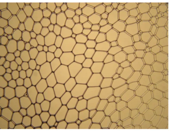
Figure 1. Recent progress in foam rheology was instigated by experiments with two-dimensional foams, obtained for example by squeezing foam between two glass plates, as in this photograph.
They include many pastes, powders, suspensions, gels and emulsions. These are generally disordered aggregates of individual entities (particles, droplets, bubbles). They may be calledBingham fluids, by reference to a particular (and rarely accurate) theoretical representation of their dual solid/liquid character.
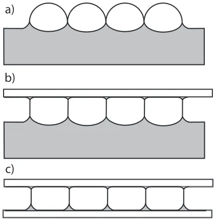
The particular appeal of foam lies in its clearly defined and simple local structure, whose rearrangements under shear may be straightforwardly characterized. It may be realized, visualized and simulated with relative ease. All of this is especially true of a two-dimensional foam, a single layer of interacting bubbles, as shown in figure 1. Such a foam may be formed in various ways; it is sometimes important to distinguish between them. It may be prepared by trapping the bubbles between two plates, or by letting them float on liquid, with or without a confining plate on top. These alternatives are illustrated in figure 2.
a)
b)
[image:3.595.200.409.93.308.2]c)
Figure 2. Three types of 2D foams: (a) monolayer of air bubbles sitting at an air/liquid interface (Bragg raft);(b)bubbles floating in liquid under a glass plate; (c) bubbles confined between two glass plates. There are large effects due to the drag associated with motion relative to solid boundaries in both (b) and (c).
by Earnshaw [4] and by Vaz and Fortes [5].
Of course, as Figure 2 makes plain, none of these foams is truly two-dimensional; nevertheless 2D models often suffice to describe their properties. Particularly when statics (or quasistatics) is all that is at stake, the differences between the three kinds of 2D foam sample may often be disregarded. However, that does not appear to be the case for 2D foam rheology, which is the topic of this review. It matters a great deal whether a confining plate is present as in Figures 2 (b) and (c).
examples of 2D foam flow, and models that represent it. Models of bubble-bubble interactions with relevance also to 3D were developed in the group of Denkov [19, 20, 21].
With benefit of hindsight, one may see that an attack on dynamical problems could have been pursued in 2D foams much earlier. It was inhibited by a vague sense that the 2D foam might not correspond well to the 3D foam whose analysis was the ultimate goal. This doubt is quite reasonable, as we shall see: nevertheless it is possible to learn a great deal from the 2D case, if it is properly understood.
In 2001 the subject was brought to a sharp focus in an experiment by Debr´egeas et al. [22]. A monolayer of bubbles, confined between two plates (as in figure 2 (c)), was introduced in a 2D cylindrical Couette viscometer of an original design. The phenomenon highlighted by the experiment was shear localization, or shear banding. When the inner cylinder was rotated, the associated shearing motion of the bubbles was restricted to a narrow region close to it. With benefit of hindsight one may discern something similar in earlier work, but here it was clearly exposed and quantified, demanding explanation. The ensuing debate has drawn in several experimental and theoretical groups, and has reached such a stage that the present topical review is justified. That is to say, much is now understood and rich detail has been revealed, but the problem remains fascinating, in that a final resolution can hardly be said to have been reached. What might have seemed a simple matter has proved to be deep and wide, causing a re-examination of foam rheology at a fundamental level. There are no further published results from the Debr´egeas instrument, but a wealth of further data has emerged from other groups, as reviewed in section 3.
Some of the main theories that are currently advanced for localization and the underlying dynamical theory arise out of the work of the Dublin [23, 24, 25, 26, 27] and Leiden [28, 29, 30] groups. This body of work, based on a continuum approximation, is not yet reconciled with alternative descriptions based an quasistatic simulations by Kabla et al. [31, 32, 33] and the Aberystwyth group [34, 35, 36]. Our first objective is to put the contributions of the Dublin and Leiden groups in the simplest complete and coherent form, as a basis for continued debate. We will however adduce some detailed simulations, in which the individual bubbles are represented, in an attempt to better understand the continuum model.
FOAM
FOAM
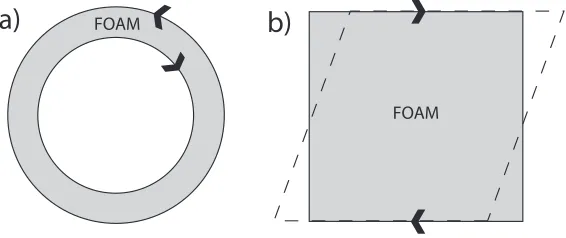
[image:5.595.165.448.96.215.2]a)
b)
Figure 3. The two types of experimental setups under consideration: (a) a circular (Couette) geometry, and (b) a straight geometry. The arrows indicate the shearing boundaries which may be displaced during an experiment or computer simulation to induce shear.
introduction of wall drag has the general consequence of shear localization, with various forms and dependencies, according to the particular case. It is therefore a crucial factor in interpreting shear localization experiments.
We will also briefly review the experimental comparisons that can be made. They largely validate the theoretical model, but additional confirmation will surely be needed, as well as further refinements of the theory.
Throughout the review we will mainly use the term shear localization, rather than shear banding. The latter term is familiar in materials science, but usually refers to localized bands of shear within the sample, whereas in the present case it is to be found only at a boundary. This distinction may be a mere matter of taste, but we prefer to avoid the connotations of the alternative expression. A more general and in many respects complementary review of “Shear Bands in Matter with Granularity” has been recently compiled by Schall and van Hecke [37].
A further type of localized deformation is possible in solid foams. Here, compression might lead to the collapse of a cell which either has a lower collapse stress or is subject to a locally higher stress [?]. This cell collapse might then propagate to cells in its vicinity, resulting in a compaction band where the cellular structure has an increased local density. Since this review article concerns liquid foams only we will not discuss such bands. In all the experiments described below the gas in the bubbles can be treated as incompressible.
If a subject is to be reviewed in the midst of its progress, all sorts of loose ends, untested assumptions and questionable generalizations will be found. On the other hand, if we wait until all is clear, it may have become stale and uninteresting! Certainly the present review falls into the “work in progress” category, and criticism will be very welcome.
We shall first review all of the main experiments and their essential results, before embarking on theoretical interpretations.
2. The experiment of Debr´egeas, Tabuteau and di Meglio
In 2001 Debr´egeas et al. noted that whereas localized shear in granular material and soil mechanics “has recently received a lot of attention from physicists [...] a clear picture has not emerged yet.” [22] They chose to work on 2D foams in the belief that “foams may shed light on the dynamics of granular systems by evidencing the minimal set of ingredients needed to get shear banding” [22]. The relationship of what is reviewed here to corresponding studies of granular systems is indeed a fascinating topic. We will comment on it only very briefly in section 16.
The apparatus consisted of a 2D circular Couette rheometer in which foam was confined between two glass plates (as in Figure 2(c)). The outer to inner radius ratio was 122mm/71mm, but note that the shear band that was eventually measured had a width of only a few millimetres. This is why the experiment can be considered equivalent to one in which simple shear is imposed and the circular geometry (which leads to a r−2
stress decay) can often be ignored, as is the case here.
The bidisperse foam was confined between plates with a separation of 2mm, and the resulting 2D bubbles had diameters only slightly greater than this (bubble diameter 2.0±0.2mmand 2.7±0.2mm respectively).
λ
*
φ
-3 -2 -1
10
0 5 15
0
10 10 10 10
r
0.1
0
0
θ
<v >
0.2 0.3
1.0 2.0 2.5
1.5
exp(-r / )λ
[image:7.595.166.432.101.291.2]φ
Figure 4. Measured velocity distributions in the original experiment by Debr´egeas et al. for Couette geometry [22]. The three different symbols mark datasets obtained for different liquid fraction. The inset shows the variation of the localization length with liquid fraction. Reprinted figure with permission from G. Debr´egeas [22]. Copyright 2001 by the American Physical Society.
of the order of 0.1s−1
within the shear band, since its width was of order of a few millimetres.
Video sequences, which were kindly made available to other groups‡, showed the process by which localization of shearing motion developed at the inner boundary, but in taking data this transient regime was avoided by allowing a full rotation before making measurements. This initial preparation corresponded to a nominal shear of the whole sample, the magnitude of which was roughly 5, and an even greater value within the region of localized shearing motion that becomes established during the rotation.
The velocity profile associated with shear localization at the moving inner boundary was consistent with an exponential form (over three orders of magnitude), that is
v(x)∝exp(−x/l), (1)
as shown in figure 4. Here l (represented by λ in the notation of these authors) is thelocalization lengthand is the main object of qualitative and quantitative scrutiny in most of the present article, although it will not always be associated with an exponential profile.
Debr´egeas et al. went on to present the variation of l with liquid fraction φ of the foam. The liquid fraction is difficult to estimate or even define satisfactorily in the present context [38]; we shall not take up this aspect of the results. Correlations of bubble motions were also analyzed.
Setting these matters aside, we may summarise some basic findings of the paper as follows.
• There islocalization at the moving boundary.
• The velocity profile has anexponential form.
• The localization length shows no variation with boundary velocity, within the range of velocities that was used.
3. Later experiments
To our knowledge, no further data has yet been reported based on the use of the particular apparatus described in the last section. Instead, various other set-ups have been employed for the same purpose, namely by the groups of Dennin and van Hecke at the universities of California-Irvine and Leiden, respectively. Here we will note the nature of these experimental variations, together with some of the key findings. A more detailed interpretation of the data is left to later sections, when its implications will be clearer.
Changes in sample geometry (from Couette to simple shear), boundary conditions, and other technical details are not generally important, but the change of foam type (among the three options of figure 2) certainly is.
3.1. Experiments by Dennin’s group using a straight geometry
diameters, independent of the velocity of the moving boundaries. (Since the applied strain rates were 0.0014, 0.0028 and 0.014 s−1
one can deduce local strain rates between 0.005 to 0.05s−1
for the sheared regions.)
The foam samples in the above experiments were nearly monodisperse (bubble diameters in the range 2.43±0.08mm) and the photo of a sample shows that the bubbles crystallize in various domains (see figure 3 of [39]). This appears to be the main contributing factor for the observed velocityindependenceof localization length in the sheared covered bubble raft. A similar behaviour for monodisperse foams was found in the experiments of the Leiden group ([28] and Section 3.3) and also in dynamic computer simulations of the viscous froth model (Section 12.3).
3.2. Experiments by Dennin’s group using Couette geometry
Dennin’s group performed further series of experiments using a Couette geometry with moving outer cylinder and bubbles in covered [43] and uncovered Bragg rafts [44, 41, 43] (Figure 2(b) and 2(c) respectively). Here the range of bubble diameter was larger than in the above experiments [39] and the issue of crystallisation should thus not arise.
Of particular relevance to the continuum theory of localization (and indeed in part inspired by this theory) are the experiments carried out in 2008 for both bubble raft and covered bubble raft in a Couette geometry with a radius ratio of 80mm/22.5mm [43]. For the bubble raft it was found that shear localizes at the inner boundary as the outer boundary was rotated. The localization length was approximately 3.5mm, independent of rotation velocity. For the covered bubble raft the localization length was found to increase with boundary velocity, from about 3mmto about 4.5mm(These widths were extracted from fits of the velocity profiles to exponentials.) Increasing the boundary velocity eventually led to the formation of a second shear band at the outer (moving) boundary. Its width was found to decrease with velocity, from about 16mm to 6mm.
4.5 5.0 5.5 6.0 6.5 0.8
1.0
4 6 8 10
0.0 0.5 1.0
v(
r
)
radial position (cm )
radial position (cm)
v(
r
[image:10.595.153.447.112.341.2])
Figure 5. Data from the Dennin group showing shear localization in the case of circular (Couette) geometry (reprinted figure 5 from [40]). The scaled azimuthal steady-state velocityv(r)/(rΩ), whereris the radial position and Ω is the rotation rate of the outer cylinder, may become constant at some internal point. In the data of [41, 42, 40], taken for a moving outer boundary and a fixed inner one, there is a discontinuity ofd(v(r)/(rΩ))/dr at this point. Note that this published figure uses the symbolv(r)to denotev(r)/(rΩ)in the notation of the present paper. The solid and dashed lines show least-square fits to power-law and exponential, respectively. This figure is used with permission from M. Dennin [40], Copyright 2008 by IOP Publishing Ltd.
section 10.
3.3. Experiments of the Leiden group
In yet another variation, the group at Leiden experimented with a bidisperse bubble monolayer (equal number of bubbles with diameter 1.8 and 2.7mmrespectively) on top of a liquid pool and covered by a glass plate (2D foam type b) of Figure 2) [28]. The distance between liquid surface and glass plate was 2.25mm. The geometry of the set-up was straight; parallel boundaries where moved at constant speed in opposite directions by two counter-rotating acrylic glass wheels, placed perpendicular to the plane of the bubble monolayer. Six different velocities were used, ranging between 0.026 and 8.4mm/s. Shear localization at the two boundaries was found to increase with velocity, as is evident in Figure 6. From the data shown one can estimate the range of applied shear rate in the respective shear bands as roughly 10−3
to 0.5s−1
[image:11.595.104.511.372.566.2]. The variation of the localization length with boundary velocity was not explicitly shown in the original publication [28]. It has since been computed by M.E. M¨obius
Figure 7. Variation of the localization length lint with wall velocity V in the Leiden experiments on bi-disperse foams [28]. The data is well described by a power law, lint ∝V−0.20, where lint is computed from a numerical integration of the measured velocity profiles, see Equation (26). The different symbols correspond to different values for the distance between the counter-rotating wheels. This figure was kindly provided by M.E. M¨obius of the Leiden group.
and is shown in Figure 7. The localization length decreases with wall velocity in the form of a power law with exponent -0.2. We will interpret this value in section 8 in terms of the continuum model.
3.4. Summary of experimental results
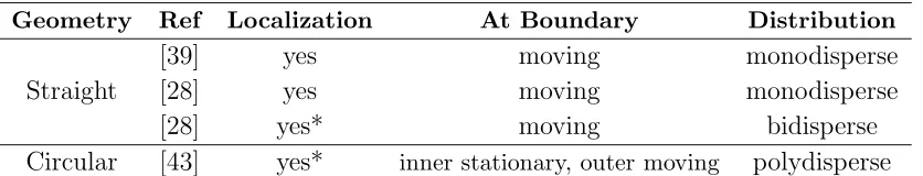
Table 1 summarises the experiments and their essential results, as regards localization. As we have seen, experimental variations include the type of 2D foam (Figure 2) and the distribution of bubble sizes (monodisperse, bidisperse, polydisperse), the geometry of the experiment (straight or Couette geometry) and the shear rates used.
SUMMARY OF EXPERIMENTS ON SHEAR LOCALIZATION
Hele-Shaw (Wall Drag)
Geometry Ref Localization At Boundary Distribution
Circular [22] yes inner moving bidisperse
Confined Bragg Raft (Wall Drag)
Geometry Ref Localization At Boundary Distribution
Straight
[39] yes moving monodisperse
[28] yes moving monodisperse
[28] yes* moving bidisperse
Circular [43] yes* inner stationary, outer moving polydisperse
Bragg Raft (No Wall Drag)
Geometry Ref Localization At Boundary Distribution
Straight [39] no - monodisperse
Circular
[44] no - tridisperse
[41] yes inner stationary polydisperse
[42] yes inner stationary polydisperse
[image:13.595.100.518.322.402.2][43] yes inner stationary polydisperse
4. Towards a theory: are 2D foam properties really similar to those of 3D foam?
We begin theoretical deliberations with the above question. When the answer isyes, this offers us one of the great simplifications of the qualitative and semi-quantitative physics of foams, extending to such subjects as structure, coarsening, elasticity and plasticity [6]. It has become almost an article of faith, but has proved misleading for rheology.
The point is simply that in most cases (including that of the seminal experiment of the Debr´egeas group [22]),the 2D foam is in contact with a solid plate. This does not matter much for static properties, but when the foam flows it entails a resisting force at the surface, which we shall here call wall drag. We shall argue that this can play a primary role in causing shear localization.
Wall drag has absolutely no counterpart in the bulk rheology of 3D foam, so it injects an essential difference into the 2D case, whenever it is present. It cannot be relevant to shear localization in three dimensions, which is sometimes seen. We shall have very little to say on that matter in the present article.
Wall drag is, in our view, essential to the analysis of shear localization in 2D, in general. There are therefore two essential ingredients to be combined in a theory: some description of theinternal forces or local rheological response of the foam, and the external drag force whenever this is present. It is absent, at least to a first approximation, in the experimental 2D system of figure 2a), but present in the other 2D foam types.
In the elementary continuum theory, it turns out that the localization length is determined by a competition between the internal dissipative forces (which tend to delocalize shear) and the external ones (which tend to enhance localization). The main theme of this article is the continuum theory that expresses this competition. By its nature it cannot capture all of the physics but, in as much as it proves to be valid, it illuminates the subject in simple terms, and makes definite predictions.
bubble diameters. These are 3D foam experiments, but there seems no reason why their implications should not extend to 2D foams as well.
5. Simulations showing shear localization
The complementary approach of detailed simulation instead of a continuum description has played an important role from the outset. In this, the detailed motion of the soap films (or other elements representative of 2D foam structure) are followed. In such a simulation the role of the local rearrangements (T1 processes) of cells can be analyzed, whereas it is buried in the empirical parameters of the continuum model.
The first theoretical analysis of the Debr´egeas experiment was based on such a 2D simulation [31] in which a 2D foam was fully represented by lines (cell walls), vertices, cell pressures etc., in a tradition dating back (at least) to the 1980s [46, 47, 48]. Two key aspects distinguish that approach from the main one considered in this article. Firstly these simulations (and various later ones [32, 33, 35]) were quasistatic, that is, they proceeded by a sequence of small changes in the boundary conditions (to represent an imposed shear), equilibrating the structure at every step. No finite shear rate is defined. Secondly, they didnot include wall drag.
It follows that in a quasistatic simulation, Galileian invariance applies: precisely the same procedure should be applicable to the natural dynamics of the system in any reference frame. In simple shear, the imposition of a velocityV at one top boundary should be entirely equivalent to the imposition of velocity −V at the opposite boundary (with zero velocity at the other boundary in each case). If localization is to be found, it ought to occur at either boundary with equal probability. This does not appear to occur in the reported results. However, in the quasistatic simulations of REF THESIS WYN, up to an applied strain of 5, the localized region is seen to slowly move between the boundaries, maintaining a roughly constant width. This might be indicative that in the quasistatic case localization is possible at both boundaries.
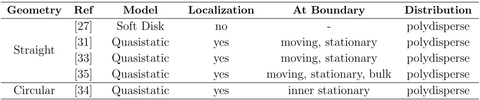
SUMMARY OF SIMULATIONS ON SHEAR LOCALIZATION
With Wall Drag
Geometry Ref Model Localization At Boundary Distribution
Straight
[27] Soft Disk yes moving monodisperse
[27] Soft Disk yes* moving polydisperse
[50] Viscous Froth yes moving monodisperse
[50] Viscous Froth yes* moving polydisperse
Circular [34] Viscous Froth yes outer moving polydisperse
Without Wall Drag
Geometry Ref Model Localization At Boundary Distribution
Straight
[27] Soft Disk no - polydisperse
[image:16.595.91.569.271.371.2][31] Quasistatic yes moving, stationary polydisperse [33] Quasistatic yes moving, stationary polydisperse [35] Quasistatic yes moving, stationary, bulk polydisperse Circular [34] Quasistatic yes inner stationary polydisperse
Table 2. Relevant detailed simulations of two-dimensional foam under shear. Categorization is by geometry and the presence or absence of wall drag. Simulations where localization length is found to depend on boundary velocity are marked with an asterix (*). Note also that many of the much earlier (1980s and 90s) simulations applied only extensional shear to the sample [48, 51, 52, 53, 54], rather than the simple shear for which localization has been observed.
In Table 2 we list relevant features and results for a variety of different detailed simulations. Viscous froth and soft disk model will be described in sections 12 and 13, respectively, and the results of these simulations will be interpreted in terms of the continuum model which we now develop.
6. Continuum theory
localization to this cause). We will not attempt to resolve it until section 10. For the meantime we pursue the course of continuum theory with wall drag, as outlined already. In this we deal with local averages of stress, strain, strain rate and related quantities, rather than the description of individual bubbles or cells. The boundary velocity V is a key parameter, in contrast to quasistatic treatments whose results are, by their very nature,V-independent.
This smoothed average picture must be questioned whenever the localization length becomes so small as to be comparable with bubble size, or according to the recent ideas of Goyon et al. [45], the range of nonlocal effects. But it seems to have a wide range of validity and is, of course, a great simplification.
6.1. Wall drag
In such a picture, the local drag force at any point~rin the moving foam contributes a body force (per unit area) F~d(~r) which is taken to be a function of local average
velocity~v(~r):
~
Fd(~r) =−cd|~v(~r)|b
~v(~r)
|~v(~r)|, (2)
with a positive drag force coefficient cd. That is, the magnitude of the drag force is
proportional to the local speed raised to the power b, and acts in direct opposition to the local velocity of the foam.
Given a power law for the drag force on one of the lines (cell walls) of Figure 1, it is obvious enough how to average it to obtain such a formula; in particular, the indexb is the same for the local force and the average. This index is not found to be unity as one might expect, and usually takes much lower values [55, 19], as explained in Section 15.
Since the average bubble motion is fixed by the direction of applied shear, we will in the following use the scalar form for the drag force (per unit area), which may be written (for positive velocity v, in the y direction, as in Figure 10 ) as
Fd(x) =−cdv(x)b. (3)
x
f
(
x
;
y,
z
)
y
z
0 1 2 3 4 5
0 0.2 0.4 0.6 0.8 1 1.2 1.4
strain
stress
limit stress yield stress
[image:18.595.161.454.98.271.2]σL σY
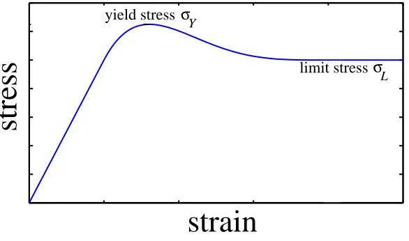
Figure 8. Quasi-static stress-strain relation with distinct yield and limit stresses, for steadily increasing strain.
6.2. Constitutive relation
The second ingredient is a local constitutive relation, relating averaged local stress, strain and strain rate. It is a traditional concept, but entails many questions and difficulties, in general.
First let us remind ourselves of the local response of a foam (3D or 2D) toslowly and steadily increasing shear (“quasistatic conditions”). It is sketched in figure 8.
For low stress or strain the foam is a linear elastic medium. In the opposite limit, as strain goes to infinity, the stress is constant. In what follows, the system will often be in the latter regime, tending to an eventual steady state in which the system is continuously sheared. Usually we shall not be concerned with the earlier transient regime.
In the model that we are developing, it is often convenient to neglect small differences between yield stress SY and limit stress SL indicated in figure 8, which
are in practice of the order of ten percent ofSY [?, 50]. Considerable simplification
is achieved in replacing the curve by a monotonic dependence of stress on (steady) strain, as in figure 9. Adopting this approach, the symbol SY stands for both yield
and limit stress, treated as identical, at least for now.
0 0.2 0.4 0.6 0.8 1 1.2
0 1 2 3 4 5
stress
σY
[image:19.595.201.407.98.253.2]strain
Figure 9. Simplified model form (expressed by the function f in the text) for a monotonic quasistatic stress-strain relation, for steadily increasing strain. No distinction is made between yield and limit stress. The functional form illustrated is that of the tanh(x) function.
for this. It increases with strain rate, but not usually in a simple linear form.
This additional stress is captured in the empirical Herschel-Bulkley relation. It is familiar in the long history of rheometry applied to 3D foams, much of it driven by industrial applications. The analysis of experimental rheological data for foams and analogous systems has been highly empirical, and has usually rested on the formalism of this relation [56]. It is just a power-law dependence of the excess stressS−SY on
strain rate ˙γ, for thesteady shear that occurs above the yield stress SY,
S =SY +cvγ˙a. (4)
Herecv is the coefficient of the viscous contribution to stress, also calledconsistency.
Often in the present article, shear is generally taken to denote local simple shear (for the somewhat subtle distinction between simple and extensional shear see [?]). The experiments cited all involvelocal simple shear but the overall macroscopic geometry of the rheometer may be straight (see Figure 3b)) or circular (Couette, see Figure 3a)).
The experiments with which we are concerned mostly involve the imposition of steady shear in one sense only. For this case one may choose to replace Equation (4) by the more general relation
S =SY f(γ/γY) +cvγ˙a, (5)
which is not confined to the steady shear state into which the system eventually settles, under an imposed strain γ > γY (γ denotes strain andγY yield strain). The
first term on the right hand side represents the dependence sketched in Figure 8 or Figure 9. This relation can be used for any imposed stress (usually constant here), such that ˙γ > 0. That is, the direction of shear cannot be reversed without modification of Equation (5).
At low strain γ, the function f(γ/γY) increases linearly with strain and
represents the (scaled) elastic stress in the linear elastic regime. In much of the work reviewed here, the function f was given a specific form such as that of the hyperbolic tangent (Figure 9).
Eventually we will have cause to revisit this simplification in search of the effects of the peak in Figure 8.
An obvious question is: how can we account for the observed values ofa? Does it reflect a corresponding dependence of local forces on local velocities? Or does it have some deeper significance? Such questions were raised in an earlier brief review [57], and part of the justification for the present one is the availability of some answers, but we will delay this discussion until section 14.
To summarise, our initial viewpoint is very restrictive and may be contrasted with that of theories that seek to develop a theory foranyarbitrarily varying imposed stress as a function of time, and more complicated geometries. Ultimately, such generality will be essential, but in the specific debate over localization it is probably unhelpful, since it would bring in an unwieldy mass of mathematical formalism.
7. Detailed results for the continuum model
• confine attention for the present to the case in which simple shear is imposed, rather than the circular or cylindrical geometry of the original experiment [22], for which it was often justifiably claimed that the geometry had little effect. We refer to this circular case as “Couette” geometry.
• set aside for the moment the detailed discussion of transient effects, that is, the evolution of motion towards the eventual steady state.
• make further approximations consistent with strong localization, that is, localization with a scale much less than that of the sample geometry. This means that the immobile boundary plays little role when the other is set in motion.
None of these simplifications are strictly required to progress the analysis but together they reduce the mathematics to a minimum, with no distracting diversions. We consider a steady state of simple shear, with an average profile v(x), as in figure 10, and will quickly show that it is localized, as illustrated.
7.1. The continuum model equation
The 2D foam is sheared by the imposition of motion at one boundary atx= 0 with velocity V, while at the other, atx=L, it is stationary (and for present arguments
L will be taken to infinity). The local strain rate is given by ˙γ =|dv(x)/dx|.
Neglecting inertia and hence equating the total force on an element to zero (as sketched in figure 11), the balance of the two forces on the element (arising from the Herschel-Bulkley relation (Equation (5)) and wall drag (Equation (3)), results in
SY
d
dxf(γ/γY) +cv d dx
d(v(x))
dx a
=−cd(v(x))b. (6)
Restricting ourselves to a discussion of the steady state at long times, the above equation is reduced to
cv cd d dx
dv(x)
dx a
=−v(x)b. (7)
We will now introduce dimensionless velocities ˆv(x), defined by
ˆ
v(x) = v(x)
v(x,t)
V
L
0
x
[image:22.595.165.448.94.282.2]y
Figure 10. Sketch of velocity profilev(x) for a straight geometry (see Figure 3b)). The foam is moved at the boundaryx= 0 with velocityV and is stationary at the boundary x=L.
d
b
c (Vv(x))
dx
d d(Vv(x))
dx
a
c
vγ γ
f( / )
Y
σ
d
dx
Y
displacement u + u
velocity v + v
∆
∆
x
∆
displacement u
velocity v
drag term
Herschel−Bulkley term
elastic/plastic term
[image:22.595.103.518.453.602.2]leading to the boundary condition ˆv(0) = 1. Thus Equation (7) is reduced to
k d dx
dˆv(x)
dx
a
=−vˆ(x)b, (9)
where the (positive) parameterk is given by
k = cv
cd
Va−b
. (10)
It contains the only dependence of the (scaled) equation on the velocity V of the moving boundary. In the following we shall proceed to solve for the steady-state profile ˆv(x) that is our concern.
Equation (9) relies on the assumption (consistent with the eventual solution given below), that everywhere dˆv
dx is negative and ˆv is positive. This avoids the
complications of hysteresis when dˆv
dx is reversed [59].
7.2. Solutions of the continuum model equation: velocity profiles
Often Equation (9) is to be solved under the boundary conditions
ˆ
v(0) = 1 and ˆv(L) = 0. (11)
However, if the profile is localized on a scale l much less than L, we may judiciously take the second condition to apply at infinity, so that
lim
x→∞vˆ(x) = 0 (12)
replaces the second part of the boundary condition (Equation (11)).
Equation (9) then has a trivial solution that may be obtained by the traditional methods applied to differential equations, or simply by inspection or trial solution, as follows. Finding the solution is complicated only by the existence of three distinct cases. (Recall thata and b are model parameters, as yet unspecified, although both are positive. Their values determine the type of solution to be applied.)
It is immediately evident that, in general, a power-law dependence of ˆv uponx
may offer a solution of Equation (9). The ansatz
ˆ
v(x) = (1−x/x0)n, (13)
0 0.2 0.4 0.6 0.8 1
0 2 4 6 8 10
velocity v(x)
position x
[image:24.595.132.472.96.339.2]a<b a=b a>b
Figure 12. Velocity profiles illustrating the three distinct cases a < b (power law),a > b(truncated power law) anda=b(exponential), where aandb are the respective exponents in Herschel-Bulkely and viscous drag relation.
For the case x0 < 0 it is acceptable for all x. We consider this case first.
Substitution into Equation (9) shows that the ansatz is indeed a solution, with the exponent n given by
n = 1 +a
a−b. (14)
The value ofx0 needs to be determined by equating prefactors, giving
a(n−1)
x0
k
n x0
a
= 1. (15)
Since x0 <0 this requires n <1, i.e. a < b. The value of x0 is given by
x0 =
1 +a a−b
a(1 +b) 1 +a k
1+1a
. (16)
Forx0 >0, the solution of Equation (9) may be developed as
ˆ
v(x) = (
(1−x/x0)n for x≤x0
0 for x > x0
(17)
wherenandx0are again given by Equation (14) and Equation (16), respectively.
However, since x0 > 0, Equation (16) requires a > b. In summary, for a > b, the
solution ˆv(x) deceases to zero at a pointx0, and is taken to be equal to zero beyond
that point. Again see figure 12.
The power law solution fails only fora=b (including the case a=b= 1, which was the original version of the continuum model [23]). In this third case the solution is exponential,
ˆ
v(x) = exp−x(ak)−1
1+a
, (18)
which may be obtained from Equation (13) by taking the limit asn tends to infinity (corresponding to (a−b)→0), or more directly by substitution.
We see that the indices a and b determine what kind of solution is found, that is;power law,truncated power law orexponential, as illustrated in Figure 12.
7.3. Definitions and results for localization lengths
What formula for the localization length emerges from these solutions? There are a number of definitions for the localization length which might be conventionally associated with a given velocity profile ˆv(x). Firstly, the internal definition for the case of exponentiallocalization, mentioned in section 2, may be generalized as
ˆ
v(le) =
1
e. (19)
(This corresponds to V /e in physical units.) In a similar manner it is possible to definel1/10,
ˆ
v(l1/10) =
1
10, (20)
or localization lengths for other fractions.
Alternatively (and equivalently to Equation (19) in the case of an exponential velocity profile) we may use
ˆ
v(0)/dvˆ dx|x=0
In the case a > b, in which ˆv(x) vanishes beyond some point x0, one could use
the smallestl for which
ˆ
v(l) = 0. (22)
This might also be applied to the case of Couette geometry, which in certain cases can provide a profile that vanishes at some point, even for a≤b [24].
For present purposes the two definitions Equation (19) and Equation (21) are preferable (with a possible third candidate which we propose for the first time below), and the choice between them is rather arbitrary.
The definition provided by Equation (21) leads to the following formula for the localisation length, arising out of the solutions developed above, and happily common to all cases (i.e. allpositive values of a and b),
l =
a(1 +b) 1 +a k
1+1a
. (23)
Recall that k is given by Equation (10) and contains a velocity dependence, so the localization length scales with velocity as
l ∝V a−b
1+a. (24)
Note also the incorporation ofcv andcdink: we see that the localization length
increases with cv and decreases with cd. When cd = 0 (no wall drag) there is no
localization. It is this statement that places the model in stark contrast to the occurrence of localization in quasistatic simulations, in which wall drag is absent.
For the case of exponential localization (a=b) Equation (23) reduces to
l =
acv cd
1+1a
. (25)
The velocity dependence of Equation (23) (contained in k, see Equation (10)) is absent, as was reported in the initial formulation of the continuum model [23].
When a localization length needs to be extracted from numerical or experimental data yet another definition may be useful, as the integration over a velocity profile reduces the effect of scatter in the data:
lint=
Z L
0
ˆ
v(x)dx. (26)
Note that lint has indeed the dimension of a length since ˆv(x) is dimensionless,
ˆ
v(x) of the continuum model (Equations (13), (17) and (18)) results in one common expression for the localization length lint. It is given, in terms of the previous
definition of l (Equations (21) and (23)), as
lint/l= (1 +a)/(1 + 2a−b). (27)
A certain amount of irreducible algebraic clutter should not detract from the very elementary nature of this treatment. It was initially developed for the casea=b = 1, leading to exponential localization, and seemed sufficient to offer an explanation of the results of Debr´egeaset al. (section 2). However, the further experiments that we have mentioned indicate the need for, at least, the solution that corresponds toa < b, leading to a decrease of localization length with boundary velocity. This arose first in the work of the Leiden group, who investigated numerical solutions of Equation (9) with finite boundary conditions corresponding to their experiments (section 3.3). Of course, all of the experiments use finite samples (finite L). The analytic solution that we have developed is for L → ∞, and nothing as simple as what we have seen emerges for finite L [26], except for the original case of a = b = 1. For this, Equation (9) is linear and has, for example, the solution in the form of a sinh function [23], appropriate to the experimental condition of figure 6 (although it was not in the end found to be applicable to that experiment).
The main qualitative conclusions of the analysis of the continuum model - that wall drag induces localization in that model (and the internal viscous dissipation opposes it) and that there is a velocity-dependence determined byaand b, must now be brought into closer contact with experiment.
8. Brief comparison with experimental data
Let us first of all examine the results which exposed a velocity dependence of localization. These were first obtained by the Leiden group, using the apparatus that we have described in section 3.3. Their model is essentially equivalent to that of the previous section, but using numerical methods and the appropriate boundary conditions fortwomoving boundaries [28, 30]. (Note however that, provided the two boundary velocities are equal and opposite, half of the system is equivalent to the case that we have chosen, by symmetry. That is, v = 0 at the midpoint.)
that is required for dragging a confined monolayer of bubbles over a smooth plate. Using this value for b (for its significance see section 15), very good agreement with observed velocity profiles was obtained for the parameter value a= 0.36.
The Leiden group also succeeded in obtaining an independent estimate of a
in reasonable agreement with these values from shearing their foam in a Couette rheometer and fitting their data to the Herschel-Bulkley model.
Using the above values for a and b in the continuum model expression for the variation of localization length with the velocity at the moving boundary (Equation (24) and Equation (27)) yields l ∝V−0.23
. This is the scaling relationship that was already shown to hold for the Leiden data (see section 3.3, Figure 7).
The further measurements of the group of Dennin added some further dimensions to our understanding. They showed that when a Bragg bubble raft is used, for which no wall drag is expected, localization is not observed [39]; this is an important element of support for the continuum model.
In these ways our understanding of shear localization in 2D foam has progressed considerably, but puzzles have remained.
• Why does the original Debr´egeas experiment show novelocity dependence? Are we to conclude that a = b in that foam sample? This remains a possibility - neither quantity was independently estimated - but it seems unlikely, in the light of other experiments.
• What is the significance of theadditional featureobserved under some conditions in Couette geometry, namely the discontinuity of the derivative of velocity profile with respect to radial position?
• How are we to resolve the apparent discrepancy between continuum modeling, and the repeated finding of localization inquasistatic simulations [31, 32, 33, 34, 35]? To clarify this issue once more, note that the V → 0 limit of continuum theory takes the localization length either to zero or to infinity, unless a = b, which we no longer consider to be correct for real foams.
9. Transient and history-dependent effects
In the original analysis of the continuum model [23], the full time-dependent form of its governing Equation (6) was used, although restricted to the case a = b = 1. Rather than finding the steady state directly, the time-dependent solution was examined for the case in which the boundary velocity is instantaneously increased from zero to the finite value V at t = 0. Steady shear is suddenly switched on, as in most experiments. This results in quite a rich scenario, in which the transient solution goes through various forms before settling down in the steady state.
Whereas the eventual steady state is described in terms of a velocity profilev(x), with the displacement profile u(x) losing any significance, we need to think of both (and indeed local strain and stress also) when dealing with the transient behaviour. Velocity and displacement are, of course, connected by v(x) = dtdu(x).
Since there has been no experimental engagement with the results, we will describe them only briefly here, referring to the original reference [23] for various diagrams that present the detail.
The boundary velocity V is switched on at t = 0, at which point it is assumed that the system is described by u =v = 0 everywhere, except at the boundary. Its response is described by the force balance equation which has the form
velocity =F(derivative of strain) +G(derivative of strain-rate) (28)
where F and G arise from the “elastic-plastic” and “viscous” terms of Equation (6), based on the Herschel-Bulkley (or in this case, Bingham, for a=1) relation. It is possible to interpret the behaviour of the system, as described by the numerical integration of Equation (6) in time, with simple mathematical arguments based on approximations, as follows.
Initially the F-term vanishes. The equation reverts to the form of Equation (9) which we have previously adduced to the steady state. Rather paradoxically, the solution immediately “jumps” to the same exponentially localized form, Equation (18).
Within the present theory this jump isinstantaneous. This cannot be physically acceptable. It is presumed that the neglect ofinertiais responsible. The propagation of a change of velocity profile on some short time-scale may be a feature of future experimental interest.
of displacement u(x), increasing from zero, and consequent strain, giving rise to a finite value of theF-term in our equation. For low enough boundary velocityV, this grows to dominate, so that the profile of v(x) and u(x) evolve from an exponential profile towards a linear form, approximating the quasi-static equilibrium solution with constant stress and strain for linear elasticity.
This form in turn is undermined by the arrival of the strain value at which the stress approaches the yield (or limit) stress. Then the elastic-plastic F-term must again diminish (eventually to zero) and the solution collapses back to its steady-state form, exponential in the present case.
This appealing scenario, in which first G, thenF, then Gagain dominates, has not yet been tested experimentally, but it does seem to correspond qualitatively to what is seen, for example, in the video of the original Debr´egeas observations‡.
More generally one may choose to implement some experimental protocol in which the boundary velocity V is some function of time. In the primitive continuum model that we have described, the steady state is unique. It is independent of the way in whichV has been varied, provided that it asymptotes to the same value. However, we shall see in section 10 that this is no longer true when certain refinements of the model are introduced, and the time-dependent equation again becomes important.
One caveat must be continually borne in mind: the equations given up to this point do not admit a reversal of the sign of the local strain-rate anywhere. This is not just conventional: hysteretic effects need to be included in the more general case.
10. Distinct yield and limit stresses
In this section we introduce an additional factor which seems necessary to fully account for the experiments. It has been recognised for a long time that the (local) yield stress, at which continuous shearing commences, is slightly greater than the eventuallimit stress. This was already sketched in Figure 8.
In previous sections this feature was not incorporated in the model. Instead the local stress was taken to be a monotonic function of strain and there was no distinction to be made between local yield and limit stresses.
Important qualitative consequences follow from having distinct yield and limit stresses. Figure 13 provides an immediate picture of what is suggested here - the
x
f
(
x
;
y,
z
)
y
z
0 1 2 3 4 5
0 0.2 0.4 0.6 0.8 1 1.2 1.4
B
A
limit stress yield stress
strain
[image:31.595.144.467.95.286.2]stress
Figure 13. The existence of distinct yield and limit stress in the quasi-static stress-strain relationship allows, at low velocities, for the coexistence of a static (corresponding to A) and a shearing region (corresponding to B). Stress at the A/B boundary is the same, due to the additional dissipative term in the shearing region.
coexistenceof static and shearing region with the same stress at the point of transition from one to the other. The effects, which are most marked below a critical boundary velocity defined below, are as follows.
• The steady state may include a part which is static, coexisting with a shearing region.
• The derivative dv
dx is finite at the boundary between shearing and static regions
(see figures 5 and 14).
• The steady state is no longer unique, but rather is dependent on history, that is, the previous variation of the boundary velocity V.
xB
static region
shearing region
x
V
v(x)
L
[image:32.595.153.464.91.278.2]B
A
Figure 14. Coexistence of sheared and static regions is possible when yield and limit stress are distinct (cf. Figure 13).
Nor is it to be confused with a similar effect for Couette geometry [24], which is induced by the circular geometry. The first clue to the necessity to refine the model was nevertheless provided by the experiments of the group of Dennin [41, 42] which had circular Couette geometry. An additional feature emerged, not predicted by that model - the finite first derivative dv
dx at the edge of the shearing region to which
we have just referred. Revisiting the original derivation of the continuum model, one may directly rule out this effect within that model, by considering the balance of forces at the point in question, separating moving and static regions. In due course, it was shown by the Dublin group [60] that replacing the elastic/plastic shape function
f(u) by one which had distinct yield and limit stresses, and proceeding as before, allowed the required feature. This interpretation was as given in figure 13. There must be equal stresses on the two sides of the boundary point between shearing and static regions, and these values correspond to the two points A and B on the diagram. In further pursuing this phenomenon, we shall revert to the straightforward case of simple shear geometry, and ask: what solutions of this kind, as in Figure 14, can exist for given V?
discussing this, we take the sample width Lto infinity, as before.
Recall that we have at our disposal the exact solution for v(x) in the limit stress regime, from Equation (9). This has a single disposable parameter which was previously fixed by the condition v → 0 as x → ∞ (the condition v(0) = 1 still holds). But now we can instead allowv to go to zero at a point xB, as in Figure 14,
proceed to examine the value of dvdx at that point, and apply the condition that stress is a continuous function of x. The solution may be stitched together at this point, provided that the viscous stress term is not too large, that is, provided that
cv|γ˙(xB)|a≤(yield stress - limit stress), (29)
at the point in question, where v is zero. For convenience, let us refer to the right hand side of Equation (29) as ∆. There is a continuous range of possible solutions defined by the above equation. For each of these we may define alocalization length l, in terms of the derivative of v at x = 0 (Equation (21)). The range of allowed solutions is illustrated by Figure 15 in terms of l, for the primitive (a = b = 1) continuum model, and another example (a= 0.5, b= 1).
In each case theuppercurvel+
(v) corresponds toxB → ∞, and it is identical to
the solution found in the earlier version of the model, with yield stress being identical to limit stress.
The lowercurvel−
(v), in which shear is most localized, has shearing and static regions (as have the solutions between the two bounds). This corresponds to equality in Equation (29). Note that it needs to be calculated numerically [50].
The range of possible solutions is large for lowV, that is, for
V <∆/√cdcv, (30)
as may be estimated by making a linear approximation for the lower values ofl close toV = 0, and finding the intersection of this with the upper curve. This value is for the primitive model (a=b= 1). For the general model it is given by [50]
V <∆aa(1++1b)
a(1 +b) 1 +a
1+1b
1
cd(cv)
1
a
!1+1b
. (31)
Having established this range of possibilities, we return to the question: which solution is selected in an experiment?
0 1 2 3 4 5
V
0 0.2 0.4 0.6 0.8 1
Localisation Length
a=1 , b=1 , cd=1 , cv=1 , ∆=1
Vc
l+(V)
l-(V)
0 1 2 3 4 5
V
0 0.5 1 1.5 2
Localisation Length
a=0.5 , b=1 , cd=1, cv=1 , ∆=1
Vc
l+(V)
[image:34.595.161.451.89.489.2]l-(V)
steady state is history-dependent [60]. The implications for future simulations and experiments are clear: the protocol of V(t) should be varied, in search for these solutions.
Before pursuing the course of detailed simulations which incorporate dissipation due to wall drag, in the next section we demonstrate that a localized solution of the kind shown above can be constructed, even if the wall drag is absent.
11. A mechanism for localization in the absence of wall drag
The present analysis has further implications for addressing the key question of: why are finite values for the localization length found in quasistatic simulations [31, 32, 33, 34, 35] when the standard continuum theory predicts otherwise?
Here we will show that the addition of the effects of the stress overshoot (see Figure 8) to the standard theory resolve this apparent discrepancy, in the limit of
V →0.
As done in Equation (6), on dimensional grounds we may relate the viscous drag force (per unit area) at point x to the local stress (a force per length in 2D) at this point:
−cdv(x)b =
dσ(x)
dx (32)
Clearly, as the boundary velocity V →0, so too does the local velocity at each point x. The left hand side of eq. 32 therefore tends to zero, leading us to the conclusion that the stress must be constant across the sample in the quasistatic regime. In a real foam, where there is a distribution of bubble sizes inducing inhomogeneity, this argument may not be accurate; but in a continuum, there are no discrete elements (bubbles), so the sample is homogenous in space.
From eq X we see that a constant stress also implies that the local strain rate is constant across the sample. This entails a linear velocity profile of the following form:
v(x) = V(1−x/l), (33)
where l is the localisation length as given by eq. 21. An example of such a velocity profile is show in Fig. 16.
Figure 16. A linear velocity profile, which occurs when the stress becomes homogeneous across the sample. l is the localisation length, which may take on a range of values (see Figure 17)
maximum possible localisation length l is the system size L. As L → ∞, this corresponds tocv|γ˙|a= 0 (see Equation (29)).
The corresponding lower bound to the range of possible localisation lengths is given bycv|γ˙|a = ∆ (see Equation (29)). From Figure??, one can see that|ǫ˙|=V /l.
Combining these two expressions leads to the following form for the localisation lengthl as a function of V:
l =cv ∆
1/a
V (34)
This gives a straight line through the origin, which intersects the (constant) upper bound at a critical velocityVc; see Figure 17. The shaded region in this figure
indicates the range of possible localisation lengths which are possible for low V. It suggests that in the quasistatic regime, the sample may adoptany localisation length between 0 and the system size L. Above the critical velocity Vc, the approximation
that the velocity profile is linear is no longer accurate however, and so the standard continuum theory applies once again.
V
Localisation Length
Vc
L
[image:37.595.178.436.94.293.2]0
Figure 17. Localisation length as a function of boundary velocityV, in the limit ofV →0. The shaded region indicates the allowable range of localisation lengths, as given by Equation (29).
yield and limit stresses is one possible mechanism for shear localisation in the absence of wall drag. Similar assertions have been made before: an argument which seems to point in the same direction is to be found in the original paper of Kabla and Debr´egeas [31].
Of particular importance here is that these arguments can be extended to 3D (where there is also no wall drag present), thereby offering a mechanism for shear localisation in this case. A detailed discussion of this phenomenon however lies outside the scope of this review article, which is concerned with shear localisation in 2D.
12. Some relevant results of the 2D viscous froth model 12.1. The model
The 2D viscous froth model was formulated quite some time ago by one of the present authors as a “toy model” of primarily theoretical interest [61, 62]. It formed a bridge between two elementary physical models that had become standard: the quasistatic equilibrium model of a dry 2D foam, and the model of curvature-driven growth of a 2D cellular structure. Indeed it contains each of these, in different limits [49].
As is so often the case, this idealised conception, initially supposed to be physically unrealistic, turned out to have a significant physical realisation. It is now a useful starting point to describe the dynamics of 2D foams and related microfluidic systems [49, 63].
The model turns the traditional static cellular model of a 2D foam, in terms of a surface tension σ and cell pressures p, into a dynamic one, by adding a viscous drag on a soap film (cell boundary), proportional to its local normal velocity. This is the “wall drag” to which we have repeatedly referred in this article, but here it relates to the detailed local motion of the soap films, rather than the average local speed of these films, as in the continuum model.
The equation of motion of a point s on a soap film is given by
λv⊥(s) = ∆p−σK(s) (35)
where λ is the drag coefficient, v⊥
(s) is the velocity in the direction normal to the boundary ats, ∆pis the pressure difference between two neighbouring bubbles,
σ is surface tension and K(s) is the local curvature, see also Figure 18.
12.2. Relationship to continuum model
The viscous froth model is a natural candidate for a dynamic simulation of 2D foam rheometry, and this has been undertaken by Barry et al. [50]. We will summarise results in Section 12.3.
Figure 18. Sketch of the forces acting on a soap film in the viscous froth model. In a computer simulation such a curved film is approximated by straight line segments and Equation (35) is applied to the end points of the segments, with the exception of the vertices.
only the wall drag term, and not the term which represents internal dissipation in the Herschel-Bulkley relation. The results will suggest otherwise.
We first address the wall drag term. A local linear drag law in the viscous froth model will give b = 1 in the continuum model, according to any simple averaging procedure. The drag constant cd of the continuum model expressed in terms of λ of
the viscous froth model may be estimated as
cd=
1 2
q
2√3 ¯A−1/2λ, (36)
where ¯Ais the mean cell area. This expression takes into account the number of cell walls per area, their average orientation, and the fact that in the continuum model the viscous drag is due only to the movement of the cell walls in the direction of applied shear [50].
of foams by the Leiden group [29].
The coefficient of the internal viscous contribution to stresscv can be written on
dimensional grounds as the following product of the parameters of the viscous froth model,
cv = ˆcvσ1
−a
λaA¯a−1/2
. (37)
Here ˆcv is a dimensionless quantity of order unity, possibly dependent on the cell size
distribution.
In the simulations, as in our previous analysis, shear is imposed on the foam by moving one boundary at velocity V, while the opposing boundary (at distance
L) is kept fixed. Soap films in contact with any of the boundaries remain in contact throughout the simulation, corresponding to no-slip boundary conditions. The overall (nominal) shear rate ˙γ is thus given by ˙γ =V /L.
Together with Equation (37) this leads to the following formulation for the Herschel-Bulkley relation in terms of the parameters of the viscous froth model,
S =SY + ˆcvσ1
−a¯ Aa−1/2
L−a
(λV)a. (38)
It is thus theproductof drag coefficient λand boundary velocity V that will play an important role when interpreting the results of the viscous froth shear simulations with the continuum model.
The immediate interest of the results may lie not so much where they conform to expectations based on elementary continuum theory but rather where they do not. For low values of the product λV there are discrepancies, which we believe are attributable to two causes.
We have already signaled one of these effects, that due to the difference of yield and limit stress (section 10). Secondly, as the effect of the drag term becomes less, the effect of disorder may become more significant, in that the yield stress may be considered to have a spatial variation.
12.3. Results of computer simulations
Figure 19. Snapshots of a shear simulation using the viscous froth model. The cell numbers help in identifying topological changes. The foam is periodic in the direction of applied shear.
of Equation (35). A velocity profile of the flowing foam is obtained by averaging the horizontal displacement of cell centres. The simulation is taken to have reached a steady state when the velocity profiles no longer appreciably change as shear is increased (this was found to require less than an applied strain of one). Steady-state velocity profiles were then averaged for values of strain between 1 and 10 and it is these steady-state profiles that were analysed for comparison with continuum theory. The simulations exhibit clear evidence of localization, as indicated by Figure 19, where the displacement of bubbles 1 to 4 in the direction of imposed shear is contrasted with that of bubbles 5 to 10 which, on average, do not move. The region of localization of flow is almost always found to occur next to the moving, as opposed to the static, boundary.
Typical velocity profiles from simulations are shown in Figure 20, for different values of λV, the product of drag coefficient λ (see Equation (35)) and boundary velocity. Localization increases withλV. §
The analytic form of the velocity profiles of Figure 20 is hard to discern from the existing simulations, due to the small system size. Future computations involving
0 2 4 6 8 10
Distance from moving boundary [A
1/2]
0 0.2 0.4 0.6 0.8 1
Average bubble velocity
λV = 0.01 σ / Α1/2
λV = 0.025 σ / Α1/2
[image:42.595.151.461.93.312.2]λV = 0.05 σ / Α1/2 λV = 0.1 σ / Α1/2
Figure 20. Velocity profiles obtained from individual viscous froth simulations using a sample of 100 cells. Increasing the product of drag coefficient λ (see Equation (35)) and velocity V of the moving boundary leads to localization near the moving boundary of the foam sample. Localization lengths can be extracted by integrating the profiles over the entire sample width, see Equation (26) and Equation (27).
larger numbers of bubbles may be more illuminating. However, it is noted that the profiles have an approximately linear form before a subsequent tail-off.
The scatter in the data makes the integral definition (Equation (26) and Equation (27)), the best choice for computing a localization lengthl. Figure 21 shows the variation of l with λV. For small values of λV there is a wide variation of the localization length l, as computed for five different realisations of foams containing 100 cells each and having a similar distribution of cell areas. As λV increases the range of l values narrows.
0 0.05 0.1 0.15 0.2 0.25 0.3
λ
V
[σ / A1/2]0 5 10
Localisation Length (l
int
-l
min)
[A
1/2
]
upper, lower bounds
Sample 1
Sample 2
Sample 3
Sample 4
Sample 5
(λV)c = 0.056
[image:43.595.139.475.95.329.2]HB exponent a = 0.3
Figure 21. Localization length for a range of values for the productλV of wall drag coefficientλand velocityV of the moving boundary. The data was computed for five different foam samples, each containing 100 cells and having a similar second moment µ2(A) of the cell area distribution (µ2(A) = 0.13±0.002). The
shaded region marks the allowed region for the localization length as given by the continuum theory for the case of distinct values for yield and limit stresses. It has been computed by setting the Herschel-Bulkely exponenta= 0.3 and the difference between yield and limit stress to ∆ = 0.11σA¯−1/2. (λV)c = 0.056σA¯−1/2 is an estimate below which value the localization length becomes essentially independent of (λV).
The upper bound for localization lengths l+
(V) (see Equation (23)) can be expressed as a function of λV by using the relevant expressions of cd and cv for the
viscous froth model (Equation (36) and Equation (37)) [50]. This results in
l+
(λV) =
2acˆvσ1
−a¯ Aa−1/2
(1 +a) ˆcd
1+1a
(λV)a−1
1+a. (39)
on Equation (31))[50]. It is given by
(λV)c =
s
2a∆1+aa( ˆcvσ1−aA¯a−1/2)−
1
a
(1 +a) ˆcd
. (40)
The above equations forl+
(λV) and (λV)c contain three unknown parameters,
namely ˆcv, ∆ and a. The difference ∆ of yield and limit stress refers to the
stress-strain curve in the quasistatic limit. It was estimated from quasistatic simulations of foams using the Surface Evolver as ∆ = 0.11σA¯−1/2
[50]. Setting the Herschel-Bulkely index to a = 0.3 and the dimensionless constant, which should be of order unity, to ˆcv = 0.26 produces both upper and lower bounds l+ and l− that look
consistent with the results from the viscous froth simulations, as shown in Figure 21 [50].
As we have already said, it is not obvious that the viscous froth model should have properties consistent with the continuum model. At this stage we can only conclude that it does, and the detailed explanation remains to be found.
13. Some relevant results of the soft disk model
Durian used a simpler, non-cellular, representation of a 2D foam, in which the bubbles are represented by overlapping disks [7, 8], as shown in figure 22. This “toy” model (equally applicable to certain granular materials) is easy to program and lends itself readily to incorporation ofad hocelastic and dissipative forces, and hence to rheology. We will call it thesoft disk modelfor present purposes.
The model has been revisited by Langlois et al. [27], and others, with startling conclusions. It appears that the approximations made by Durian and others in the very early attempts at such a simulation were such as to render some of the results erroneous.
velocity V
Figure 22. Snapshot of a shear simulation using the disk model. In the example shown the bubbles are confined between a static boundary aty= 0 and a moving boundary aty=H [27]. The simulation uses periodic boundary conditions in the x-direction only.
13.1. Definition of the model
The forces in the soft disk model are as follows. When two disks (representing two bubbles) overlap (and only then) they interact via a simple spring force, the displacement of the spring being the radial overlap (see Fig. 23).
The elastic repulsive forceFn acting on bubble i (centred atri, with radius Ri)
due to bubble j (centered at rj, with radius Rj) is then given by
Fn =κ 2R0
Ri+Rj
∆ijnij. (41)
Hereκ is the coefficient of elasticity, nij is the normal vector between bubbles i and j,
nij=
ri−rj |ri−rj|
, (42)
and the overlap ∆ij is given by
∆ij =
(
(Ri+Rj)− |ri−rj| if (Ri +Rj)<|ri−rj|
R
R
r
r ∆
i
i j j
[image:46.595.241.369.99.238.2]ij
Figure 23. Overlap ∆ij between two contacting bubbles of radii Ri and Rj, located at riandrj, respectively.
(see Fig.23). The ratio 2R0
Ri+Rj in Equation (41), where R0 is the average bubble
radius of the entire bubble packing, takes into account that larger bubbles are easier to deform than smaller ones.
A real flowing foam dissipates energy by viscous friction in the films and Plateau borders separating the bubbles. The simplest expression, as used by Durian [8] and [27], represents the viscous force Fb on bubble i associated with a neighbouring bubblej as
Fb =−cb(vi−vj) (44)
wherecb is the dissipation constant for the bubble-bubble interaction and vi and vj are the respective bubble velocities.
Wall drag in the case of a foam confined between two plates adds an additional force on all moving bubbles. It is given by
Fwd(r) =−cwd|v(r)|b
v(r)
|v(r)|, (45)
where cwd is the wall drag constant. The exponent b = 1 in the simulations of
Langloiset al.
![Figure 4. Measured velocity distributions in the original experiment by Debr´egeaset al.obtained for different liquid fraction.localization length with liquid fraction.for Couette geometry [22].The three different symbols mark datasetsThe inset shows the var](https://thumb-us.123doks.com/thumbv2/123dok_us/969472.610177/7.595.166.432.101.291/measured-distributions-experiment-dierent-localization-fraction-dierent-datasetsthe.webp)
![Figure 5. Data from the Dennin group showing shear localization in the case ofcircular (Couette) geometry (reprinted figure 5 from [40])](https://thumb-us.123doks.com/thumbv2/123dok_us/969472.610177/10.595.153.447.112.341/figure-dennin-showing-localization-ofcircular-couette-geometry-reprinted.webp)
![Figure 6.The Leiden experiment [28].between a liquid pool and a covering glass plate. (b) Localization takes place closeto the moving boundaries, the localization length decreases with boundary velocity.Reprinted figures with permission from M](https://thumb-us.123doks.com/thumbv2/123dok_us/969472.610177/11.595.104.511.372.566/experiment-localization-boundaries-localization-decreases-reprinted-gures-permission.webp)
![Figure 7. Variation of the localization length lint with wall velocity V in theLeiden experiments on bi-disperse foams [28].The data is well described by apower law, lint ∝ V −0.20, where lint is computed from a numerical integration ofthe measured velocit](https://thumb-us.123doks.com/thumbv2/123dok_us/969472.610177/12.595.133.480.87.337/variation-localization-theleiden-experiments-described-numerical-integration-measured.webp)