Piecewise Multi-Linear Model Based Control for TORA System via Feedback Linearization

Piecewise Multi-Linear Model Based Control for

TORA System via Feedback Linearization

Tadanari Taniguchi and Michio Sugeno

Abstract—This paper deals with a piecewise model based controller design for nonlinear systems via feedback lineariza-tion. The model is a piecewise multi-linear system and a nonlinear approximation. The approximated model is fully parametric. Feedback linearization is applied to stabilize PML (Piecewise Multi-Linear) control system. We apply the piecewise model based controller to TORA (Translational Oscillator with Rotating Actuator) system. Although the controller is simpler than the conventional feedback linearization controller, the PML model based control can be applied to a wider region than the conventional one. Examples are shown to confirm the feasibility of our proposals by computer simulations.

Index Terms—nonlinear control, feedback linearization, tora system, piecewise model.

I. INTRODUCTION

W

E propose a piecewise model based controller de-sign for nonlinear systems via feedback linearization. We apply the piecewise model based controller to TORA (Translational Oscillator with Rotating Actuator) system. The TORA system [1] has a cart of mass M connected to a wall with a linear spring (constantk). The cart can oscillate without friction in the horizontal plane. A rotating mass m

in the cart is actuated by a motor. The mass is eccentric with a radius of eccentricity eand can be imagined to be a point mass mounted on a massless rotor. The rotating motion of the massm controls the oscillation of the cart (see Fig. 2). TORA system is difficult to control because the system has a complex nonlinear dynamics.

Many methods have been studied for the stabilizing control of TORA system. The exact feedback linearization method is proposed in [1]. However the controller is limited in the angle of the rotor. The cascade and passivity based control designs is proposed in [2]. This method can be applied to the limited region of the state variable. The model-based fuzzy controls are proposed in [3], [4].

In this paper, we consider piecewise multi-linear (PML) model as a piecewise approximation model of TORA system. The model is built on hyper cubes partitioned in state space and is found to be bilinear (bi-affine) [5], so the model has simple nonlinearity. The model has the following features: 1) The PML model is derived from fuzzy if-then rules with singleton consequents. 2) It has a general approxima-tion capability for nonlinear systems. 3) It is a piecewise nonlinear model and second simplest after the piecewise linear (PL) model. 4) It is continuous and fully parametric. The stabilizing conditions are represented by bilinear matrix inequalities (BMIs) [6], therefore, it takes long computing

Manuscript received January 5, 2018; revised January 31, 2018. This work was supported by Grant-in-Aid for Scientific Research (C:26330285) of Japan Society for the Promotion of Science.

T. Taniguchi is with IT Education Center, Tokai University, Hiratsuka, Kanagawa, 2591292 Japan email:[email protected]

M. Sugeno is with Tokyo Institute of Technology.

time to obtain a stabilizing controller. To overcome these difficulties, we have derived stabilizing conditions [7], [8], [9] based on feedback linearization, where [7] and [9] apply input-output linearization and [8] applies full-state linearization. The control system has the following features: 1) Only partial knowledge of vertices in piecewise regions is necessary, not overall knowledge of an objective plant. 2) Although the structure of the PML controller is very simple, the PML control system can be applied to a wider region than the feedback linearization [1].

This paper is organized as follows. Section II introduces the canonical form of PML models. Section III briefly presents TORA system. Section IV presents a stabilizing con-troller design using exact feedback linearization. Section V-VI propose a PML modeling and a PML model based control for TORA system via exact feedback linearization. Section VII shows some examples demonstrating the feasibility of the proposed methods. Finally, section VIII summarizes conclusions.

II. CANONICALFORMS OFPIECEWISEMULTI-LINEAR MODELS

A. Open-Loop Systems

In this section, we introduce PML models suggested in [5]. We deal with the two-dimensional case without loss of generality. Define vectord(σ, τ)and rectangleRστ in two-dimensional space asd(σ, τ)≡(d1(σ), d2(τ))

T ,

Rστ ≡[d1(σ), d1(σ+ 1)]×[d2(τ), d2(τ+ 1)]. (1)

σ and τ are integers: −∞ < σ, τ < ∞ where d1(σ) <

d1(σ+ 1), d2(τ)< d2(τ+ 1)andd(0,0)≡(d1(0), d2(0))T. SuperscriptT denotes atranspose operation.

We consider a two-dimensional nonlinear system:

˙ x=f(x)

Forx= (x1, x2)∈Rστ, the PML system is expressed as

            

˙

x=fp(x) = σ+1

X

i=σ τ+1

X

j=τ

ω₁i(x1)ω2j(x2)f(i, j),

x=

σ+1

X

i=σ τ+1

X

j=τ

ω₁i(x1)ω j

2(x2)d(i, j),

(2)

wheref(i, j)is the vertex of nonlinear systemx˙ =f(x),

                        

ω₁σ(x1) =

(d1(σ+ 1)−x1)

(d1(σ+ 1)−d1(σ))

,

ω₁σ+1(x1) =

(x1−d1(σ))

(d1(σ+ 1)−d1(σ))

,

ω₂τ(x2) =

(d2(τ+ 1)−x2)

(d2(τ+ 1)−d2(τ))

,

ω₂τ+1(x2) =

(x2−d2(τ))

(d2(τ+ 1)−d2(τ))

and ωi 1(x1), ω

j

2(x2) ∈ [0, 1]. In the above, we assume

f(0,0) = 0andd(0,0) = 0to guarantee x˙ = 0 forx= 0. A key point in the system is that state variable xis also expressed by a convex combination of d(i, j) for ωi

1(x1) andωj₂(x2), just as in the case ofx˙. As seen in equation (3),

x is located inside Rστ which is a rectangle: a hypercube in general. That is, the expression of x is polytopic with four vertices d(i, j). The model of x˙ =f(x) is built on a rectangle includingxin state space, it is also polytopic with four verticesf(i, j). We call this form of the canonical model (2) parametric expression.

B. Closed-Loop Systems

We consider a two-dimensional nonlinear control system.

(

˙

x=f(x) +g(x)u(x),

y=h(x). (4)

For x ∈ Rστ, the PML model (5) is constructed from a nonlinear system (4).

(

˙

x=fp(x) +gp(x)u(x),

y=hp(x),

(5)

where

                                    

fp(x) = σ+1

X

i=σ τ+1

X

j=τ

ω₁i(x1)ω2j(x2)f(i, j),

gp(x) = σ+1

X

i=σ τ+1

X

j=τ

ω1i(x1)ω2j(x2)g(i, j),

hp(x) = σ+1

X

i=σ τ+1

X

j=τ

ω₁i(x1)ω j

2(x2)h(i, j),

x=

σ+1

X

i=σ τ+1

X

j=τ

ω₁i(x1)ω2j(x2)d(i, j),

(6)

and f(i, j), g(i, j), h(i, j) and d(i, j) are vertices of the nonlinear system (4). The modeling procedure in regionRστ is as follows:

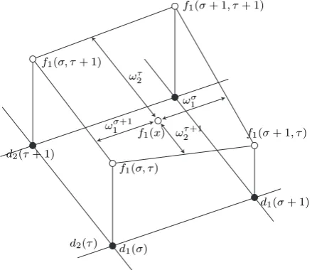
1) Assign verticesd(i, j)forx1=d1(σ),d1(σ+1),x2=

d2(τ),d2(τ+ 1)of state vector x, then partition state space into piecewise regions (see Fig. 1).

2) Compute verticesf(i, j),g(i, j)andh(i, j)in equation (6) by substituting values ofx1=d1(σ),d1(σ+1)and

x2=d2(τ),d2(τ+1)into original nonlinear functions

f(x),g(x) and h(x)in the system (4). Fig. 1 shows the expression off1(x)andx∈Rστ.

The overall PML model is obtained automatically when all vertices are assigned. Note that f(x), g(x)andh(x)in the PML model coincide with those in the original system at vertices of all regions.

III. TORASYSTEM

The TORA (Translational Oscillator with Rotating Actua-tor) system [1] has a cart of massM connected to a wall with a linear spring (constant k). The cart can oscillate without friction in the horizontal plane. A rotating mass m in the cart is actuated by a motor. The mass is eccentric with a radius of eccentricity e and can be imagined to be a point mass mounted on a massless rotor. The rotating motion of the

d1(σ)

d1(σ+ 1)

d2(τ) d2(τ+ 1)

f1(σ+ 1, τ)

f1(σ, τ) f1(σ, τ+ 1)

f1(σ+ 1, τ+ 1)

ω₁σ+1

ωσ₁

ω₂τ+1 ωτ

2

[image:2.595.327.547.53.243.2]

f1(x)

Fig. 1. Piecewise region (fp1(x) =

Pσ+1 i=σ

Pτ+1 j=τω

i 1ω

j

[image:2.595.311.548.496.589.2]

2f1(i, j),x∈ Rστ)

Fig. 2. Kinematic model of TORA system

massmcontrols the oscillation of the cart. The motor torque is the control variable. The dynamics of TORA system is

                    

˙ z1=z2

˙ z2=

−z1+εz24sinz3

1−ε2_cos2_z 3

− −εcosz3 1−ε2_cos2_z

3

v

˙ z3=z4

˙ z4=

1 1−ε2_cos2_z

3

εcosz3 z1−εz24sinz3+v

y=z1,

(7)

where z1 and z2 are the position and velocity of the cart.

z3=θ andz4= ˙θare the angle and angular velocity of the rotor. The parameterεdepends on the eccentricityeand the massesM andm.v andy are the control input and output.

The TORA system dynamics has many nonlinear terms. In the case of a coordinate transformation

x1=z1+εsinz3

x2=z2+εz4cosz3

x3=z3

x4=z4

u=εcosz3(x1−εsinz3(1 +z

2 4)) +v

1−ε2_cos2_z 3

we have

          

˙

x=f+gu=

   

x2

−x1+εsinx3

x4

0

   

+

   

0 0 0 1

   

u

y=h=x1,

(8)

wherex∈R4_,y∈R.

IV. CONTROLLER DESIGN OFTORASYSTEM VIA EXACT FEEDBACK LINEARIZATION

We design the controller of TORA system (8) via the exact feedback linearization [10]. We calculate the time derivatives of the output y until the inputuappears.

y=h=x1,

˙

y=Lfh=x2

y(2)=L2_fh=−x1+εsinx3

y(3)=L3_fh=−x2+εcosx3

y(4)=L4_fh+LgL3fhu

=x1−εsinx3−εx42sinx3+εcosx3u

Then the controller is obtained as

u=−L

4 fh

LgL3f

+ 1

LgL3f

µ

=−x1+εsinx3+εx

2 4sinx3

εcosx3

+ 1

εcosx3

µ, (9)

whereµis the linear controller for the linearized system (10).

( _˙

ξ=Aξ+Bµ

y=Cξ, (10)

whereξ= (h, Lfh, L2fh, L 3 fh)

T_,

A=

   

0 1 0 0

0 0 1 0

0 0 0 1

0 0 0 0

   

, B=

   

0 0 0 1

   

, C=

   

1 0 0 0

   

T

.

However the controller (9) is only well defined at −π/2< x3 < π/2 because the denominator of the controller is

εcosx3. Hence the rotor of TORA system can only be rotated at−π/2< θ < π/2.

V. PML MODEL OFTORASYSTEM

We construct the PML model of TORA system (8). The nonlinear term sinx3 of TORA system is transformed into a PML model representation. The variable of x3 is divided by m vertices x3 ∈ {d3(1), d3(2), . . . , d3(m)}. For x3 ∈

{d3(σ), d3(σ+ 1)}, the PML model is expressed as

          

˙

x=fp+gpu=

   

x2

−x1+εfp2(x3)

x4

0

   

+

   

0 0 0 1

   

u

y=hp=x1,

(11)

where

fp2(x3) = σ+1

X

i=σ

w₃i(x3)fs(i), fs(i) = sind3(i),

ωσ₃(x3) =

(d3(σ+ 1)−x3)

(d3(σ+ 1)−d3(σ))

,

ωσ+1₃ (x3) =

(x3−d3(σ))

(d3(σ+ 1)−d3(σ))

.

σis integer: −∞< σ <∞,d3(σ)< d3(σ+ 1). The PML model is constructed with respect tofp2(x3) = sinx3. The structure is independent of the state variablesx1,x2 andx4 since the variables are the linear terms.

Note that trigonometric functions of TORA system (7) are smooth functions and are of class C∞. The PML models are not of class C∞. In TORA system control, we have to calculate the fourth derivatives of the outputy. Therefore the derivative PML models lose some dynamics. However the PML model based control for TORA system can be applied to a wider region than the conventional one.

VI. PMLMODEL BASED CONTROL FORTORASYSTEM VIA EXACT FEEDBACK LINEARIZATION

We define the output asy=x1in the same manner as the previous section, the time derivative ofy is calculated as

˙

y=Lfphp=x2

The time derivative of y doesn’t contain the control inputs

u. We calculate the time derivative of y˙. We get

¨

y=L2_fphp=fp2(x1, x3) =−x1+ε σ+1

X

i=σ

wi₃(x3)fs(i),

wherex3∈ {d3(σ), d3(σ+1)}. The time derivative ofy˙also doesn’t contain the control inputsu. We continue to calculate the time derivative ofy¨. We get

y(3)=L3_f

php=−x2+ε

fs(σ+ 1)−fs(σ)

d3(σ+ 1)−d3(σ)

x4

We continue to calculate the time derivative ofy(3)_{. We get}

y(4) =L4_fphp+LgpL

3 fphpu

=x1−ε σ+1

X

i=σ

wi₃(x3)fs(i) +ε

fs(σ+ 1)−fs(σ)

d3(σ+ 1)−d3(σ)

u

The stabilizing controller of (11) is designed as

u= −L

4 fphp

LgpL

3 fphp

+ 1

LgpL

3 fphp

µ

= x1−ε

σ+1

X

i=σ

wi₃(x3)fs(i)

εfs(σ+ 1)−fs(σ) d3(σ+ 1)−d3(σ)

+ 1

εfs(σ+ 1)−fs(σ) d3(σ+ 1)−d3(σ)

µ (12)

wherex3 ∈ {d3(σ), d3(σ+ 1)} andµ=−F ζ is the linear controller of the linear system (13).

( _˙

ζ=Aζ+Bµ,

y=Cζ, (13)

whereζ = (hp, Lfphp, L

2 fphp, L

3 fphp)

T_{. The parameters}

Iffs(i)6=fs(i+ 1) andd3(i)6=d3(i+ 1),i= 1, . . . , m, there exists a controller (12)u of TORA system (11) since

det(LgpL

3

fphp) 6= 0. Thus we have to construct the PML

model of TORA system such that fs(i) 6= fs(i+ 1) and

d3(i)6=d3(i+ 1), where i= 1, . . . , m(see Fig. 3).

1

0 x3

(d3(3), fs(3))

(d3(4), fs(4))

π/2 (d3(5), fs(5))

fs(x3) = sinx3

[image:4.595.313.540.80.352.2]

fs(4)−fs(3)) d3(4)−d3(3)

Fig. 3. PML modeling

Note that the PML model based controller (12) can be applied to a wider region than the conventional feedback linearized controller (9).

VII. SIMULATION RESULTS

We apply the feedback linearization controller (9) and the PML model based controller (12) to TORA system (7) in a computer simulation. We can select the arbitrary position and the arbitrary number of the vertices d3(i) in

x3. Although there are some modeling errors because the PML model is a nonlinear approximation, it is possible to adjust the approximated error. In the following simulations, the parameter εis 0.5.

A. The difference between with the number of divided regions The state variable x3 of TORA system (8) is divided by four regions (x3 ∈ {−π, −π/2, 0, π/2, π}) to construct the PML model. We consider the feedback gain

F = (1.000, 3.078, 4.236, 3.078) such that the lin-earized control system (13) is stable. The initial condition is x(0) = (1, 0, 0, 0)T_{. Fig. 4 shows that the control} system is unstable because of the model approximation error. Therefore the state variable x3 is divided by eight regions (x3 ∈ {−π, −3π/4, −π/2, . . . , π}) to construct the PML model. Next the state variable x3 is divided by 16 regions (x3∈ {−π, −7π/8, −3π/4, . . . , π}) to construct the PML model. It is enough to select the PML model divided by eight regions from the results of Figs. 5 and 6.

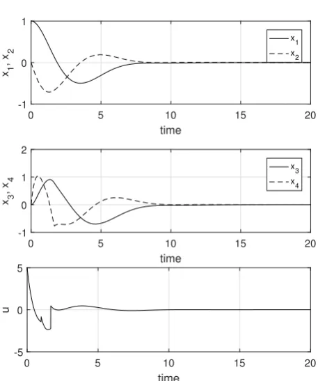
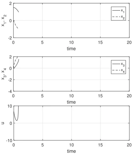
B. Exact feedback linearization and PML model based con-trol

For an exact feedback linearized control and the PML model based control, we use the feedback gains F = (1.000, 3.078, 4.236, 3.078) and the initial conditions

x(0) = (1.5,0,0,0)T. Fig. 7 shows the exact feedback linearized control responses. The control and the input re-sponses are stopped at a time whenx3> π/2. Fig. 8 shows

0 5 10 15 20

time

-1 0 1

x 1

, x

2

x 1 x

2

0 5 10 15 20

time

-1 0 1 2

x 3

, x

4

x 3 x

4

0 5 10 15 20

time

-5 0 5 10

u

Fig. 4. Control and input responses of PML model based control with four regions

0 5 10 15 20

time

-1 0 1

x 1

, x

2

x₁ x₂

0 5 10 15 20

time

-1 0 1 2

x 3

, x

4

x 3 x

4

0 5 10 15 20

time

-5 0 5

u

[image:4.595.51.289.126.313.2] [image:4.595.312.541.445.719.2]

0 5 10 15 20

time

-1 0 1

x1

, x

2

x 1 x

2

0 5 10 15 20

time

-1 0 1

x3

, x

4

x₃ x

4

0 5 10 15 20

time

-5 0 5

[image:5.595.54.285.52.314.2]

u

Fig. 6. Control and input responses of PML model based control with 16 regions

the control results when the state variable x3 is divided by eight regions (x3 ∈ {−π, 3π/4, . . . , π}) to construct the PML model. The controller achieves stabilizing control at the external region of kx3k ≤π/2.

0 5 10 15 20

time

-2 0 2

x1

, x

2

x 1 x

2

0 5 10 15 20

time

-4 -2 0 2

x3

, x

4

x₃ x

4

0 5 10 15 20

time

-10 0 10

u

Fig. 7. Exact feedback linearization

VIII. CONCLUSIONS

This paper has proposed a piecewise model based con-troller design for nonlinear systems via feedback lineariza-tion. We have applied the piecewise model based controller

0 5 10 15 20

time

-2 0 2

x 1

, x

2

x 1 x

2

0 5 10 15 20

time

-4 -2 0 2

x 3

, x

4

x₃ x₄

0 5 10 15 20

time

-10 0 10

[image:5.595.312.540.52.313.2]

u

Fig. 8. PML model based control

to TORA system. Although the controller is simpler than the conventional feedback linearization controller, the PML model based control can be applied to a wider region than the conventional one. Examples have been shown to confirm the feasibility of our proposals by computer simulations. We will verify the robust performance and design an H∞ controller in the future works.

REFERENCES

[1] R. Sepulchre, M. Jankovic, and P. Kokotovic,Constructive Nonlinear Control. Springer, 1997.

[2] M. Jankovic, D. Fontaine, and P. Kokotovic, “Tora example: cascade and passivity based control designs,”IEEE Transactions on Control Systems Technology, vol. 4, no. 3, pp. 292–297, 1996.

[3] K. Tanaka, T. Taniguchi, and H. O. Wang, “Model-based fuzzy control of tora system: fuzzy regulator and fuzzy observer design via lmis that represent decay rate, disturbance rejection, robustness, optimality,” in

IEEE World Congress on Computational Intelligence, 1998. [4] Lon-ChenHung, H. P. Lin, and H. Y. Chung, “Design of self-tuning

fuzzy sliding mode control for tora system,” Expert Systems with Applications, vol. 32, no. 1, pp. 201–212, 2007.

[5] M. Sugeno, “On stability of fuzzy systems expressed by fuzzy rules with singleton consequents,”IEEE Trans. Fuzzy Syst., vol. 7, no. 2, pp. 201–224, 1999.

[6] K.-C. Goh, M. G. Safonov, and G. P. Papavassilopoulos, “A global optimization approach for the BMI problem,” inProc. the 33rd IEEE CDC, 1994, pp. 2009–2014.

[7] T. Taniguchi and M. Sugeno, “Piecewise bilinear system control based on full-state feedback linearization,” inSCIS & ISIS 2010, 2010, pp. 1591–1596.

[8] ——, “Stabilization of nonlinear systems with piecewise bilinear models derived from fuzzy if-then rules with singletons,” in FUZZ-IEEE 2010, 2010, pp. 2926–2931.

[9] ——, “Design of LUT-controllers for nonlinear systems with PB models based on I/O linearization,” inFUZZ-IEEE 2012, 2012, pp. 997–1022.

[image:5.595.54.285.425.691.2]