Polymer Bonded Explosives 1 pdf

On predicting the effective elastic properties of polymer

bonded explosives using the recursive cell method

Biswajit Banerjee

_{, Daniel O. Adams}

Department of Mechanical Engineering, University of Utah, 50 S Central Campus Drive, 2120 MEB, Salt Lake City, UT 84112, USA

Received 22 December 2002; received in revised form 8 September 2003

Abstract

Polymer bonded explosives are particulate composites containing elastic particles in a viscoelastic binder. The particles occupy an extremely high fraction of the volume, often greater than 90%. Under low strain rate loading (0.001–1 s1_{) and at room temperature and higher, the elastic modulus of the particles can be four orders of}

mag-nitude higher than that of the binder. Rigorous bounds and analytical estimates for the effective elastic properties of these materials have been found to be inaccurate. The computational expense of detailed numerical simulations for the determination of effective properties of these composites has led to the search for a faster technique. In this work, one such technique based on a real-space renormalization group approach is explored as an alternative to direct numerical simulations in determining the effective elastic properties of PBX 9501. The method is named the recursive cell method (RCM). The differential effective medium approximation, the finite element method, and the generalized method of cells (GMC) are investigated with regard to their suitability as homogenizers in the RCM. Results show that the RCM overestimates the effective properties of particulate composites and PBX 9501 unless large blocks of subcells are ren-ormalized and the particles in a representative volume element are randomly distributed. The GMC homogenizer is found to provide better estimates of effective elastic properties than the finite element based homogenizer for composites with particle volume fractions less than 0.80.

2003 Elsevier Ltd. All rights reserved.

Keywords:Particulate composites; Elastic properties; Renormalization; Generalized method of cells; Finite elements

1. Introduction

One of the goals of multi-scale modeling of materials is to predict the behavior of these materials across many different length scales. These length scales range from the atomistic (nanometers) to the macroscopic (meters). Many multi-scale simulations move from a smaller scale to a larger one by using coarse-grained representations of the material and its microstructure in the larger scale. Micromechanics provides a process by which coarse-graining can be achieved by producing effective properties that can be used in the macroscopic simulations.

*

Corresponding author. Tel.: +1-801-585-5239; fax: +1-801-585-9826. E-mail address:[email protected](B. Banerjee).

0020-7683/$ - see front matter2003 Elsevier Ltd. All rights reserved. doi:10.1016/j.ijsolstr.2003.09.016

For two-phase random composite materials with relatively low volume fractions of the dispersed phase (<0.50), excellent estimates of the effective elastic properties can be obtained from micromechanics-based rigorous bounds or analytical approximations. However, such estimates are grossly inaccurate for par-ticulate composites containing extremely high volume fractions of particles and strong modulus contrasts between the phases. This is especially true for polymer bonded explosives (PBXs) which can have particle volume fractions greater than 0.90 and modulus contrasts between particles and binder greater than 20,000. For PBX 9501, third-order upper and lower bounds on effective moduli can be three orders of magnitude apart and analytical estimates can be an order of magnitude different from experimental values.

In the absence of close bounds and accurate analytical approximations (Banerjee and Adams, in press), the prediction of effective properties of PBXs requires numerical simulations that explicitly consider the microstructure of the composite. However, direct numerical simulations are computationally expensive. Such simulations become prohibitive when the effective properties of the composite are to be computed in the course of a multi-scale simulation.

Methods derived from the real-space renormalization group (RSRG) (Wilson, 1971a, 1979) have been found to provide an accurate means of determining certain effective properties of materials (such as con-ductivity, permeability, etc.) with relatively low computational cost. The recursive cell method (RCM) attempts to apply the idea of renormalization to the determination effective elastic properties of high volume fraction and high modulus contrast particulate composites such as PBXs.

The idea behind renormalization is that, in a large system, local high frequency oscillations of a state variable do not influence the low frequency behavior of the system. Thus, if a method can be found that accurately averages out the local fluctuations, then a larger system can be built with the averaged local regions as the building blocks. This idea is implemented in the RCM by dividing the representative volume element (RVE) into subcells using a regular grid. Small blocks of subcells are then homogenized in a re-cursive manner until an effective property of the composite is obtained. The homogenization of blocks of subcells is performed using finite elements, the generalized method of cells (GMC) or any other suitable technique. For simplicity, only two phase particulate composites are considered in this work. However, the number of phases is not limited in any way by the method.

The organization of this paper is as follows. Section 2 discusses the rationale behind using RSRG approaches for high volume fraction particulate composites. The RCM is described in Section 3 and homogenization techniques appropriate to this method are presented. Section 4 provides background in-formation on PBXs and PBX 9501, bounds and analytical estimates of the effective properties of PBX 9501, followed by a brief discussion of the difficulties associated with direct finite element and generalized method of cells analyses of PBX microstructures. Predictions from the RCM using different homogenizers are discussed in Section 5. Finally, the results are summarized and conclusions presented in Section 6.

2. Renormalization

The original use of the renormalization group (RG) occurs in quantum electrodynamics (Stueckelberg and Petermann, 1953; Gell-Mann and Low, 1954; Wilson, 1971a,b). The goal in that context was to replace the fine structure of point masses and charges with observable quantities. The RG is a group GðTsÞof transformations Tsthat take a pointxn2Rþinto the point xnþ12Rþ(in one dimension) in such a way

that

xnþ1¼xnfðCnþ1=Cn;xnÞ xnfðs;xnÞ; ð1Þ

whereCn, Cnþ1 are constants that couple the two points,f is a function of sand xn. Then, the

transformation inverse T_s1. The transformation is usually nonlinear, unlike the deformation gradient tensor in finite elasticity.

The RSRG was originally proposed by Kadanoff (Wilson, 1971a). The idea of RSRG methods is to consider a material to be divided into blocks containingN3_{cells (or lattice sites). Each block of material is}

then considered to act as a unit (a single effective material) in a new, scaled lattice. The new set of cells (or lattice sites) are again divided into blocks and subjected to the same process until a fixed point is obtained. The fixed point is that situation in which each block has the same material properties. If we consider a lattice model of an elastic solid, the RSRG approach consists of a set of transformationsT Tsthat take a

lattice of spacing l with probability density PnðK;lÞinto another lattice of spacing a lwith probability density

Pnþ1ðK;lÞ ¼TðPnðK;lÞÞ; ð2Þ

whereKis the bulk modulus,lis the shear modulus,Pnþ1is the probability distribution of elastic properties

on the new lattice, andPn is the probability distribution on the old lattice.

The probability distributionsP and the transformation T are usually not amenable to analytical rep-resentation. Hence, an approximate method is usually used to determine the discrete distribution of properties on the lattice at each recursion. The RVE that is homogenized using this approach is assumed to be considerably larger than the size of individual subcells. Therefore, scale similarity arguments can be used to justify the used of a RSRG approach if the RVE is infinite compared to each subcell. In numerical RSRG approaches, an infinitely sized RVE is not possible to simulate. Instead a finite sized RVE is chosen and scale similarity is assumed to exist in that RVE. A complete review of numerical RSRG approaches is outside the scope of this work. However, we will try to motivate and explore the applicability of one such approach to PBX materials.

Standard homogenization theories average all the fluctuations in the RVE in a single step usually using a perturbation-based approach. Such effective medium theories lead to unreasonable effective properties when the fluctuations are large and rapid, as is the case in high modulus contrast/high volume fraction particulate composites (Banerjee and Adams, in press).

In contrast, RSRG approaches smooth out the local fluctuations at each step (nþ1) of the recursion after a detailed computation at the initial step (n1). The physical argument that is used to justify this

ap-proach is that local fluctuations in the properties do not propagate their effects to the long range. This argument requires that length scales in the problem are well separated.

Renormalization-based techniques have been widely used for studying critical phenomena in percolating systems (Feng and Sahimi, 1985; Stauffer and Aharony, 1992) including elastic networks (Feng and Sahimi, 1985). Other applications to percolating systems include the calculation of the effective conductance of lattices (Bernasconi, 1978) and composites (Shah and Ottino, 1986), the effective permeability of rocks (King, 1989), effective dispersivities of flows (Jaekel and Vereecken, 1997), the effective hydraulic con-ductivity of heterogeneous media (Hristopulos and Christakos, 1999; Renard et al., 2000), and the effective elastic properties of porous media (Poutet et al., 1996).

The similarity of PBXs to percolating systems is that stress is transported mainly (but not exclusively) through contact between particles (Bardenhagen et al., 2001), in a manner analogous to percolation through the material. If the RVE is large enough, the local length scales are well separated from macro-scopic scales. This consideration has motivated the use of a RSRG method to estimate the effective properties of PBXs. An additional incentive is that RSRG methods are considerably faster than conven-tional numerical averaging methods because the whole domain is not homogenized at a time. Instead, some averaging is done at a smaller length scale and the average properties are appropriately scaled for use at a larger length scale.

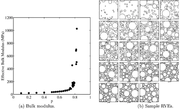
using detailed finite element analyses of square RVEs containing circular particles in a continuous binder. The particle size distribution is based on that of the dry blend of PBX 9501 (Skidmore et al., 1997). More information of PBX 9501 is given in Section 4.

The Youngs modulus of the particles is 25,000 MPa while that of the binder is 1 MPa. The Poissons ratio of the particles is 0.20 and that of the binder is 0.49. The bulk moduli are approximately 14,000 MPa for the particles and 2 MPa for the binder. The finite element homogenization approach and its conver-gence behavior have been described in detail elsewhere (Banerjee et al., 2003). A brief description in the context of the RCM is provided in Section 3.2. All material properties used as inputs to the models in what follows are three-dimensional properties. Also, all comparisons are made between three-dimensional properties.

Ninety-four randomly generated microstructures (similar to those shown in Fig. 1(b)) have been used to calculate the effective bulk moduli shown in Fig. 1(a). From the figure, it can be observed that the per-colation threshold is around 0.80 for such composites. PBXs with volume fractions >0.90 lie near this threshold. This suggests that the transport of stress through PBXs is analogous to transport through percolating networks and similar techniques may be used to study the features of both PBXs and perco-lating networks.

3. The recursive cell method

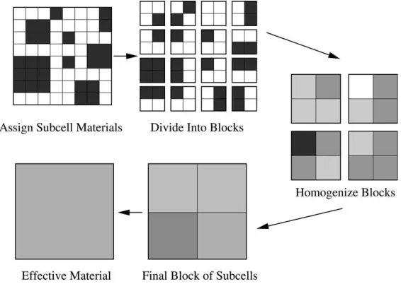
A schematic of the RCM is shown in Fig. 2. The RCM approach requires the RVE to be initially discretized into a regular grid of subcells. The subcells are assigned material properties depending on the particle distribution in the RVE. The subcells in the original grid are grouped into blocks ofNNsubcells. The effective elastic properties of each block are calculated using an approximate homogenization tech-nique, e.g., using an effective medium approximation, a lattice spring model, the finite element method, the generalized method of cells or combinations of these methods. These stiffnesses are then assigned to a new, coarser grid.

In standard renormalization approaches, the above process is repeated until a ‘‘fixed point’’ is reached where the effective properties of all the blocks have the same value. However, in the simulations performed

in this work, the recursion terminates when only one homogeneous block remains after a fixed number of iterations since the domain is finite. The properties of this homogeneous block are assumed to be the effective properties of the RVE. For simplicity, only two-dimensional models of particulate composites and PBX 9501 are considered in this paper. Extension of RCM to three-dimensions follows the same procedure and is straightforward.

3.1. Differential effective medium homogenization

In this section, we discuss how a differential effective medium theory (D-EMT) can be used to homo-genize a block in RCM. The usual D-EMT (Markov, 2000; Garbozci and Berryman, 2001 and references therein) procedure is as follows. Suppose particles with elastic moduliKp andlp are embedded in a binder

with elastic moduliKbandlb. Suppose that a dilute volume fractionpof particles have been placed in the

binder. The effective moduli Keff and leff of the resulting composite are computed using the dilute

ap-proximation. The resulting composite is treated as a homogeneous material with moduli equal to the computed moduli. Suppose then that more particles are added by removing a differential volume (dV) from the composite, and replacing it with an equivalent volume of particles. The new composite properties can again be calculated using the dilute limit. As dV !0, the process can be approximated by the following coupled differential equations for the effective elastic moduli,

ð1pÞdKeff

dp ¼ ðKpKeffÞ

Keffþ4=3leff

Kpþ4=3leff

; ð3Þ

ð1pÞdleff

dp ¼ ðlpleffÞ

leffþueff

Kpþueff

; ð4Þ

where,pis the volume fraction of particles, K is the bulk modulus andl is the shear modulus. The sub-scripts (p) and (eff) denote particles and the composite, respectively, and

ueff¼ ðleff=6Þð9Keffþ8leffÞ=ðKeffþ2leffÞ: ð5Þ

In the context of RCM, the D-EMT has to be applied sequentially for each inclusion material in a block of subcells. The volume fraction of each material in a block is determined by the number of subcells oc-cupied by the material. The most compliant material is assumed to be the binder. The D-EMT approach is used to calculate the effective composite properties as each of the stiffer materials is sequentially added to the binder. The final effective property is assigned to the block of subcells and the process is repeated for the next level of recursion. It should be noted that the sequence of addition of materials can determine the final values of the effective properties of the composite. Also, any anisotropy in the distribution of particles in the RVE is ignored by the D-EMT approximation.

3.2. Finite element homogenization

An alternative to D-EMT homogenization is to use the finite element method (FEM) for direct nu-merical homogenization. In this section, we describe a FEM approach Bathe (1997) for calculating the effective elastic properties of blocks of subcells.

We use two-dimensional, plane strain, finite elements that avoid numerical integration to homogenize blocks of subcells. RSRG methods are quite sensitive to approximation errors (Renard et al., 2000). However, accurate FEM calculations for blocks of subcells with large modulus contrasts require conside-rable discretization of each subcell and hence involve large computational cost. Instead, we model each subcell using one nine-noded displacement based element (for particles), or one nine-noded mixed dis-placement/pressure based element (for the binder). Explicit forms of the strain–displacement and stress– strain relations are used to arrive at explicit forms for stiffness matrices (see Appendix A) and average stresses and strains in each element.

Periodic displacement boundary conditions are applied to each block of subcells (see Appendix B). The state of stress is calculated using FEM for an applied homogeneous normal or shear strain. The average stresses and strains in a block of subcells are then used to determine the effective stiffness matrix for the block using the relation

Z

V

rijdV ¼Ceff

ijkl

Z

V

kldV; ð6Þ

whereV is the volume of the block,Ceff

ijkl is the effective elastic stiffness tensor of the composite,rijare the

stresses, andij are the strains.

The process is repeated after all the blocks at each level of recursion have been assigned effective stiffness matrices. The effective moduli of the RVE are calculated after the effective stiffness matrix has been de-termined for the final level of recursion. At this stage, the RVE is assumed to be isotropic and the following procedure is followed.

For the two-dimensional case, the effective stiffness matrix of the RVE is of the form

C¼

Ceff

11 Ceff12 0

Ceff 12 C

eff 22 0

0 0 Ceff

66

2 4

3

5: ð7Þ

The approximate effective two-dimensional Youngs modulus (E2D

eff) and Poissons ratio (m 2D

eff) are

cal-culated using the relations

m2D eff ¼2C

eff 12=ðC

eff 11 þC

eff 22Þ; E

2D

eff ¼0:5ðC eff 11 þC

eff 22Þ½1 ðm

2D effÞ

2

: ð8Þ

We assume that the composite is isotropic and that the two-dimensional properties to have been ob-tained from plane strain calculations. The three-dimensional Youngs modulus (Eeff), Poissons ratio (meff),

meff ¼m2Deff=ð1þm 2D

effÞ; Eeff ¼Eeff2D½1 ðmeffÞ 2

; Geff ¼Eeff=½2ð1þmeffÞ: ð9Þ

3.3. Generalized method of cells homogenization

The GMC (Paley and Aboudi, 1992) is another technique that has been used to calculate the effective properties of composites. When GMC is used as the homogenizer in RCM, a block of subcells is homogenized in a single step without explicit calculation of the stresses in the block. Thus, each block of subcells is considered to be a RVE in the GMC sense and periodic boundary conditions are applied implicitly to the block.

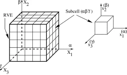
A brief description of the two-dimensional GMC follows. Fig. 3 shows a schematic of the RVE, the subcells and the notation (Aboudi, 1991) used in GMC. In the figure, (X1;X2) is the global coordinate

system of the RVE andðxð₁aÞ;xð₂bÞÞis the local coordinate system of the subcellðabÞ.

It is assumed that the displacement functionuð_iabÞvaries linearly within a subcellðabÞand can be written in the form

u_iðabÞðx₁ðaÞ;xð₂bÞÞ ¼wð_iabÞðX1;X2Þ þUðiabÞx

ðaÞ

1 þH

ðabÞ

i x

ðbÞ

2 ; ð10Þ

whereirepresents the coordinate direction and takes the values 1 or 2, andwð_iabÞis the mean displacement at the center of the subcellðabÞ. The constantsUð_iabÞandHð_iabÞrepresent gradients of displacement across the subcell. The strain–displacement relations for the subcell are given by

ð_ijabÞ¼1

2 oiu ðabÞ

j

þoju

ðabÞ

i ; ð11Þ

whereo1¼o=ox

ðaÞ

1 ando2¼o=ox

ðbÞ

2 .

If each subcell ðabÞ has the same dimensions ð2h;2hÞ, then the average strain in the subcell can be obtained in terms of the displacement field variables using Eqs. (10) and (11), and

hð_ijabÞiV ¼

1 4h2

Z h

h

Z h

h

ð_ijabÞdx₁ðaÞdxð₂bÞ: ð12Þ

We assume continuity of traction at the interface of two subcells. In addition, displacements and tractions are assumed to be periodic at the boundaries of the RVE. Applying the displacement continuity equations on an average basis over the interfaces between subcells, the average strain in the RVE can be expressed in terms of the subcell strains. The average subcell stresses can be obtained from the subcell

strains using the traction continuity condition and material stress–strain relations. A relationship between the subcell stresses and the average strains in the RVE is thus obtained.

For transversely isotropic or isotropic materials, the above approach leads to decoupled systems of equations for the normal and shear response of the RVE. The system of equations for the normal stresses and strains are of the form,

M11 M12

M21 M22

T1

T2

¼ H

0 h11iV þ 0

H h22iV; ð13Þ

wherehiV represents an average over the whole RVE.

The corresponding system of equations for the shear components are

M4T12¼Hh12iV: ð14Þ

In Eqs. (13) and (14) theMmatrices contain material compliance terms. TheTmatrices contain the average subcell stresses. The vector H contains the dimensions and number of subcells. After inverting these equations, explicit algebraic expressions are obtained relating the average RVE stresses to the average RVE strains. These equations are of the form

hr11iV hr22iV hr12iV

2 4

3

5¼

Ceff

11 Ceff12 0

Ceff

12 Ceff22 0

0 0 Ceff

66

2 4

3

5 h

11iV h22iV

2h12iV

2 4

3

5; ð15Þ

whereCeff

ij are the terms of the effective stiffness matrix. Details of the algebraic expressions for these terms

can be found elsewhere (Pindera and Bednarcyk, 1997).

Due to decoupling of the normal and shear response of the RVE, the shear components of the stiffness matrix obtained from GMC are the harmonic means of the subcell shear stiffnesses and of the form

1=C₆₆eff¼1=N2X

N

a¼1

XN

b¼1

1=Cð₆₆abÞ; ð16Þ

whereN is the number of subcells per side of the RVE.

Once the stiffness matrix for a block of subcells has been calculated using GMC, the procedure is re-peated recursively to get the effective stiffness of the RVE. The effective stiffness is then converted into moduli using the assumption of isotropy and Eqs. (8) and (9).

The shear modulus predicted by GMC is equal to the harmonic mean of the shear moduli of the subcells. This error can be ignored if the effective elastic properties of a particulate composite are computed from the normal components of the stiffness matrix.

4. Polymer bonded explosives

4.1. Properties of PBX 9501 and constituents

PBX 9501 is a PBX containing monoclinic crystals of high melting explosive (HMX) dispersed in a viscoelastic binder which is a 1:1 mixture of a rubber (Estane 5703) and a plasticizer (bis dinitropropy-lacetal/formal––BDNPA/F). Since the HMX crystals are randomly oriented in PBX 9501, isotropic elastic properties can be used while modeling the particles in the composite.

Experiments on HMX (Zaug, 1998) show an average Youngs modulus (E) of 15.3 GPa and a Poissons ratio (m) of 0.32. Molecular dynamics simulations (Sewell and Menikoff, 1999) predict a Youngs modulus of 17.7 GPa and a Poissons ratio of 0.21 for HMX.

Experiments on the binder in PBX 9501 show temperature and strain rate dependence of elastic pro-perties. The binder has a Youngs modulus of approximately 0.7–1 MPa at low strain rates (0.001–1 s1₎

(Cady et al., 2000). The Youngs modulus of HMX is around 20,000 times that of the binder at these strain rates. At high strain rates (1500–3500 s1_{), the Youngs modulus of HMX is around 10–20 times that}

of the binder. The binder modulus decreases with increase in temperature. Since the binder is rubbery, it is assumed to have a Poissons ratio of 0.49.

The Youngs modulus of PBX 9501 at low strain rates is approximately 1 GPa, and at high strain rates around 5–7 GPa (Gray III et al., 1998). The Poissons ratio of PBX 9501 is around 0.35 (Wetzel, 1999).

4.2. Particle size distribution in PBX 9501

The dry blend of HMX particles in PBX 9501 is a mixture of two different size distributions of particles. The coarse HMX particles are sized between 44 and 300lm while the fine particles are less than 44lm. The particles are mixed in a 3 to 1 ratio of coarse to fine particles. In the composite, the smaller particles fit into the interstitial spaces between the larger ones.

The manufacture of PBX 9501 involves mixing the dry blend of HMX and the binder to form molding powder granules of PBX 9501. These powders are then isostatically compressed at 90C until the porosity is reduced to 1–2% and the pressed form of PBX 9501 is obtained. The size distribution of HMX particles in PBX 9501 after processing is significantly different from that before processing (Skidmore et al., 1997). The cumulative volume fraction of the finer sized particles is dramatically higher in pressed PBX 9501 compared to the dry blend. Fig. 4(a) shows the particle size distributions of HMX in the dry blend and the pressed piece. A sample microstructure of PBX 9501 is shown in Fig. 4(b).

4.3. Bounds, analytical, and direct numerical estimates for PBX 9501

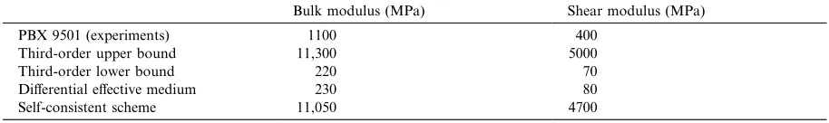
Table 2 shows third-order bounds and some analytical estimates for the effective bulk and shear moduli of PBX 9501 at low strain rate and room temperature. Rigorous third-order bounds (Milton, 1981) on the effective elastic properties of PBX 9501 at low strain rates can be observed to be considerably far apart. Commonly used analytical approximations such as the differential effective medium approximation (DEM)

Table 1

Typical polymer bonded explosives (Gibbs and Popolato, 1980)

PBX Explosive particle Binder

Material Volume fraction Material Volume fraction

PBX 9010 RDX 0.87 KEL-F-3700 0.13

PBX 9501 HMX 0.92 Estane 5703 + BDNPA/F 0.08

and the self-consistent scheme (SCS) (Markov, 2000) are also observed to provide inaccurate estimates for the elastic moduli of PBX 9501.

Direct numerical estimates of the effective elastic moduli of PBX 9501 have been discussed elsewhere (Banerjee, 2002). Direct finite element estimates have been found to require considerable computational expense because of the high degree of discretization required.

5. Estimates from the recursive cell method

In this section, estimates of effective moduli are obtained for RVEs containing 10–92% by volume of circular particles. These estimates show the performance of RCM both above and below the percolation threshold of0.80. Next, RCM is applied to models of PBX 9501 and the estimated moduli are compared with experimental data. Finally, some convergence properties of the method are explored and the strengths and weaknesses of the method are identified.

5.1. Models of random particulate composites

Fig. 5 shows two-dimensional RVEs of random composites containing circular particles. The volume fractions of particles vary from 0.10 to 0.92. The particle size distribution is roughly based on the particle size distribution of HMX in the dry blend of PBX 9501 (see Fig. 4(a)).

Fig. 4. Particle size distributions in the dry blend of PBX 9501 and in pressed PBX 9501 and the microstructure of PBX 9501 (adapted from Skidmore et al., 1997, 1998).

Table 2

Bounds and analytical estimates of the effective elastic properties of PBX 9501

Bulk modulus (MPa) Shear modulus (MPa)

PBX 9501 (experiments) 1100 400

Third-order upper bound 11,300 5000

Third-order lower bound 220 70

Differential effective medium 230 80

A Youngs modulus of 100 GPa and a Poissons ratio of 0.20 were assigned to the particles. The Youngs modulus of the binder was varied from 1 MPa to 10 GPa in multiples of 10 while the Poissons ratio was kept fixed at 0.49.

The effective Youngs moduli of these RVEs have been calculated using RCM with different homoge-nizers. For this purpose, each RVE was discretized into 256·256 subcells. For the initial iteration, a subcell was assigned particle properties if it was found to contain >50% particles by volume. Otherwise the sub-cell was assigned binder properties. RCM estimates were obtained using blocks of 2·2 and 16·16 sub-cells, respectively.

To compare the RCM results with estimates from direct numerical simulations, plane strain finite ele-ment analyses were performed with each subcell being represented by a four-noded eleele-ment. Periodic displacement boundary conditions were used to determine the average stresses and strains in the direct finite element computations. The effective moduli were calculated using the approach discussed in Section 3.2.

An extra set of calculation were performed with a binder Youngs modulus 1 MPa so that convergence of the direct finite element calculations could be verified. In these direct FEM computations, each subcell of the RVE was modeled using a eight-noded quadrilateral element. Table 3 shows the values of effective modulus from four-noded and eight-noded computations. Eight-noded elements lead to lower effective moduli than four-noded elements. However, the difference is within 6% for volume fractions less than 0.80.

Fig. 5. RVEs containing 10–92% by volume of circular particles.pis the volume fraction of particles in a RVE.

Table 3

Comparison of effective Youngs moduli from direct FEM calculations using four-noded and eight-noded elements

Volume fraction 0.10 0.20 0.30 0.40 0.50 0.60 0.70 0.79 0.92

Four-noded element (66 049 nodes)

Modulus (MPa) 1.3 1.9 2.6 3.8 5.7 9.8 19.4 95.1 3542.3

Eight-noded element (197 633 nodes)

Modulus (MPa) 1.3 1.8 2.6 3.7 5.4 9.4 18.3 89.2 2991.7

The difference is 15.5% for the RVE containing 92% particles, primarily because the stress concentrations at particle contacts that dominate the calculation are not well resolved with four noded elements.

Fig. 6 shows the calculated effective Youngs modulus of the nine RVEs as a function of volume fraction and modulus contrast. Note that the computed values at binder volume fractions of 0 and 1 are exact when computed using RCM (for all three homogenizers).

5.1.1. RCM with D-EMT homogenizer

The first set of RCM computations were performed using a D-EMT homogenizer (RCMD-EMT) as

discussed in Section 3.1. Estimates using blocks of 2·2 subcells are shown in Fig. 6(a). Those using blocks of 16·16 subcells are shown in Fig. 6(b). The sequence of addition of materials in the D-EMT has been chosen to be in ascending order of Youngs modulus. Use of other sequences leads to a difference of less than6% in the estimated effective modulus of the microstructures considered.

From Fig. 6(a) it can be seen that the RCMD-EMTcalculations predict values that are less than the direct

FEM estimates. Qualitatively, the difference is small for low particle volume fractions but is considerable for the volume fractions of 0.80 and 0.92. For example, for the volume fraction of 0.92 and binder modulus of 10 MPa, the RCMD-EMT estimate is 1.3 GPa while the direct FEM estimate is 7 GPa. The difference

grows larger when 16·16 subcells are used to homogenize a block (as shown in Fig. 6(b)). In that case, the RCMD-EMT estimate is 0.6 GPa. It should be noted that the RCMD-EMT estimate is closer to the

experi-mental value for PBX 9501 and may actually be the better estimate.

5.1.2. RCM with FEM homogenizer

The second set of RCM computations were performed using a FEM homogenizer (RCMFEM) as

dis-cussed in Section 3.2. Estimates using blocks of 2·2 and 16·16 subcells are shown in Fig. 6(c) and (d), respectively. The RCMFEMestimates have been obtained from calculations in which each subcell in a block

was modeled using a square, nine-noded, displacement based element.

The RCMFEMestimates with 2·2 subcells per block are almost an order of magnitude higher than the

direct FEM estimates for all volume fractions and modulus contrasts shown in Fig. 6(c). When the number of subcells in a block is increased to 16·16, the estimates are closer to FEM predictions, especially for low modulus contrasts. These results suggest that further discretization of each block of subcells is required for RCMFEMto predict moduli that are closer to direct FEM estimates.

5.1.3. RCM with GMC homogenizer

One of the reasons for the high RCMFEM estimates is the low number of degrees of freedom in each

block of subcells. However, increased discretization of a block of subcells decreases the computational efficiency of RCM. Since the GMC requires less discretization than finite elements for the same accuracy (Aboudi, 1996), RCMGMC can be used for improved accuracy without significant loss of computational

efficiency.

Since the displacement based FEM predicts elastic properties which are upper bounds (Banerjee, 2002), it is also possible that the overestimation of elastic properties by RCMFEM is due to the accumulation of

errors from both the FEM approximation and the renormalization technique. In this regard, since GMC predicts lower bounds on elastic properties (Banerjee, 2002), it is possible that predictions from RCMGMC

would improve over those from RCMFEMbecause errors due to renormalization cancel out approximation

errors in GMC.

The third set of RCM computations were performed using a GMC homogenizer (RCMGMC) as discussed

in Section 3.3. Fig. 6(e) and (f) show the moduli from RCMGMC calculations using blocks of 2·2 and

16·16 subcells, respectively.

The RCMGMC estimates using blocks of 2·2 subcells are closer to the FEM estimates of Youngs

modulus than the RCMFEM results shown in Fig. 6(c). However, these estimates are considerably higher

than the FEM and RCMD-EMT predictions. When the subcells/block in a block is increased the RCMGMC

estimates improve. There are some pathological cases in which the error in the predicted modulus is higher than average (for the RVEs containing particle volume fractions of 0.50, 0.70 and 0.80). Considerably improved RCMGMCestimates are obtained when 16·16 subcells are used to form a block, as shown in

Fig. 6(f). In that case, the RCMGMC estimates are within a few percent of the direct FEM predictions

It is interesting to note that the number of subcells per side (16), at which RCMGMC provides good

estimates, can be expressed as N1=d_{, whereN is the total number of subcells, and d is the dimensionality}

of the problem. Further exploration of this observation has not been carried out at this time.

5.1.4. Computational expense

The direct FEM calculations on the RVEs (discretized into 256·256 four-noded elements) using ANSYS 6.0 (ANSYS, 2002) take around 150 CPU seconds on a SunSparc Ultra-60 with 512 Mb RAM running Solaris 7. All the RCM programs were coded in Java using JDK 1.4. The 16·16 subcells/block RCMD-EMT

calculations took around 10 CPU seconds to compute. The corresponding RCMFEM calculations take

around 130 CPU seconds, while RCMGMC takes around 140 CPU seconds.

Thus, even the 16·16 subcell RCMGMC calculations provide a slight improvement in efficiency over

direct finite element calculations. In addition, the 16·16 subcell RCMGMCprovides a means of computing

accurate effective properties for RVEs of high particle volume fraction particulate composites that need to be discretized considerably. In such cases, though direct finite element calculations may not be possible due to limitations on the available computational power, the effective properties of the RVE can be obtained using RCMGMCcalculations on smaller blocks of the whole RVE.

5.2. Models of PBX 9501

A sample microstructure of PBX 9501 is shown in Fig. 4(b). The particles in the microstructure are irregularly shaped and of a large number of sizes. The volume fraction of particles in PBX 9501 is around 92%. A digital image of the microstructure is difficult to simulate since particles and binder are not easily distinguished. Instead, models containing circular particles with particle size distributions that correspond to that of PBX 9501 have been used to model the PBX.

The four microstructures shown in Fig. 7(a) are based on the particle size distribution of the dry blend of PBX 9501 (see Fig. 4(a)). The microstructures contain 100, 200, 300, and 400 particles, respectively. The corresponding RVE sizes are 0.65, 0.94, 1.13, and 1.325 mm. The particles in the microstructures occupy about 86% of the volume.

Microstructures based on the particle size distribution of pressed PBX 9501 are shown in Fig. 7(b). The four microstructures contain 100, 200, 500, and 1000 particles respectively. The corresponding RVE sizes are 0.36, 0.42, 0.535, and 0.68 mm. The particles occupy 89%, 87%, 86% and 85.5% of the volume, re-spectively. Higher volume fractions could not be achieved using the random sequential particle addition technique used. Also, particle sizes below 9lm have not been used because they fall below the resolution of the computational grid.

Since actual PBX 9501 contains 92% particles, the remainder of the particle volume fraction is incor-porated into adirtybinder. For example, the dirty binder in the models shown in Fig. 7(a) contains about 30% fine HMX particles and 70% binder. The D-EMT approach was used to determine the elastic pro-perties of the dirty binder.

The model RVEs in Fig. 7 were discretized into 256·256 subcells. Subcells containing more than 50% binder by volume were assigned dirty binder properties while those containing less than 50% binder were assigned particle properties. Note that this discretization and material assignment is also necessary for direct finite element computations since it is not possible to create elements of acceptable shape at the point of contact of two circular particles.

A Youngs modulus of 15.3 GPa and a Poissons ratio of 0.32 was used for the particles. These are the moduli of HMX at room temperature. The Youngs modulus of the pure binder is 0.7 MPa and the Poissons ratio is 0.49 at a temperature of 25C and a strain rate of 0.01 s1_{. The elastic moduli of the dirty}

(1.6 MPa, 0.484) for model PP1, (2.1 MPa, 0.481) for model PP2, (2.7 MPa, 0.478) for model PP3, and (3.0 MPa, 0.477) for model PP4.

The effective moduli of the RVEs were calculated with RCM using 16·16 subcells/block. As a check, direct FEM estimates of the moduli were also obtained. These FEM calculations were performed by treating each subcell as an eight-noded element (197,633 nodes in the mesh). Table 4 shows the effective Youngs moduli and Poissons ratios of the models of PBX 9501 from RCM and direct FEM calculations. The ratio of the RCM estimates to the direct FEM estimates are also given as a measure of error, assuming that the direct FEM calculations are accurate.

For the models based on the dry blend, the RCMD-EMTcalculations predict Youngs moduli that are less

than 4% of the direct FEM estimates. This result can be expected based on the results shown in Fig. 6(b). The RCMFEMestimates vary from 160% to 260% of the FEM values. This result also reflects the data for

random particulates shown in Fig. 6(d). From the results shown in that figure, one should expect that, of the three homogenizers, the 16·16 RCMGMC calculations to provide the best estimates of the effective

Youngs modulus. However, this trend is not observed for the RCMGMCestimates shown in Table 4.

From the table, it can be seen that the RCMGMCestimates are between 7% and 15% of the FEM values,

whereas the results in Fig. 6(f) show that GMC results are within 90% of the FEM values for the particulate RVEs considered. The same trends are observed from the data shown in Table 4 for the models of pressed PBX 9501. These results suggest that the effect of contact between particles is not being captured correctly by RCMGMC, especially when such interactions dominate the material response.

5.2.1. Direct FEM computations

At this stage, it is of interest to check whether the direct FEM computations have converged to a stable value, whether the FEM predictions would decrease with further mesh refinement, and if the FEM pre-dictions are close to the experimentally determined moduli of PBX 9501.

Table 5 shows the results obtained from direct FEM computations for the eight model PBX 9501 microstructures. Errors with respect to a PBX 9501 Youngs modulus of 1.0 GPa and a Poissons ratio of 0.35 are also shown in the table.

The table shows that a threefold increase in the number of nodes leads, except in two cases, to a decrease of 10–15% in the effective Youngs modulus. The Poissons ratio does not appear to be affected significantly by mesh refinement. The effective Youngs modulus does not always decrease with mesh refinement for the models of PBX 9501 unlike the models of random composites (see Table 3).

This discrepancy may indicate a lack of convergence of the FEM computations on the models of PBX 9501. It is conceivable that further refinement would lead to improved solutions. However, the associated computational cost is very high and further mesh refinement has not been explored except for one model (PP4). For model PP4, each subcell was subdivided into four eight-noded displacement elements (800,000 nodes). FEM computations using this grid led to values of moduli that are only 3% lower than those using200,000 nodes. Hence, we may assume that the FEM computations have probably converged.

The use of generalized plane strain elements leads to lower values of Poissons ratios indicating a stiffer lateral response than that using plane strain elements. The lower Youngs moduli suggest a more compliant response in the direction of the applied strain. However, the difference between the plane strain and the generalized plane strain predictions is not large enough to warrant the extra computations required for the latter case.

Table 4

Effective moduli of PBX 9501

Model Youngs modulus (GPa) Poissons ratio

DB1 DB2 DB3 DB4 DB1 DB2 DB3 DB4

Models of PBX 9501 dry blend

RCMD-EMT 0.05 0.06 0.10 0.09 0.40 0.38 0.37 0.37

RCMFEM 4.59 4.34 4.84 6.12 0.17 0.15 0.20 0.21

RCMGMC 0.12 0.32 0.16 0.42 0.32 0.19 0.29 0.15

Direct FEM 1.76 2.08 2.54 3.84 0.22 0.23 0.25 0.25

RCMD-EMT/

FEM

0.03 0.03 0.04 0.02 1.8 1.7 1.5 1.5

RCMFEM/

FEM

2.6 2.1 1.9 1.6 0.8 0.7 0.8 0.8

RCMGMC/

FEM

0.07 0.15 0.06 0.11 1.4 0.8 1.2 0.6

PP1 PP2 PP3 PP4 PP1 PP2 PP3 PP4

Models of pressed PBX 9501

RCMD-EMT 0.07 0.10 0.14 0.15 0.38 0.36 0.35 0.34

RCMFEM 5.45 4.97 6.69 7.25 0.17 0.18 0.22 0.24

RCMGMC 0.13 0.23 0.24 0.20 0.33 0.22 0.21 0.26

Direct FEM 2.60 2.97 4.65 5.34 0.23 0.21 0.25 0.26

RCMD-EMT/

FEM

0.03 0.03 0.03 0.03 1.7 1.7 1.4 1.3

RCMFEM/

FEM

2.1 1.7 1.4 1.4 0.7 0.9 0.9 0.9

RCMGMC/

FEM

The mixed displacement/pressure elements provide the lowest values of effective Youngs modulus. The error involved in using such elements, which are accurate for nearly incompressible materials, does not seem to be large enough to warrant their use either.

It is also observed that the models of PBX 9501 do not reflect the correct behavior of PBX 9501. The predicted Youngs moduli of the dry blend models are between 70% and 300% higher than the moduli of PBX 9501. The comparisons are worse for the models of pressed PBX 9501––between 160% and 440% higher. There could be several possible causes for the discrepancy, some of which are listed below.

(1) The materials model used for HMX, the binder, and/or PBX 9501 are incorrect. The effective elastic properties of thermoviscoelastic materials cannot be obtained without taking the loading history into consideration.

(2) The use of circular particles is inappropriate. The actual shapes of the particles have to be modeled. (3) The dirty binder model is incorrect. The actual volume fraction of particles needs to be modeled. (4) The particle size distribution in the models is incorrect, especially after the RVE has been discretized

and materials assigned using the 50% rule.

(5) The use of a two-dimensional plane strain model leads to artificially high effective moduli.

(6) A square RVE is inappropriate for the calculation of isotropic properties. RVEs with hexagonal sym-metry should be used.

(7) The RVEs are too small to represent PBX 9501. Larger RVEs with better discretization are needed.

Table 5

Effective moduli of PBX 9501 from direct FEM calculations

Element Nodes Youngs modulus (GPa) Poissons ratio

DB1 DB2 DB3 DB4 DB1 DB2 DB3 DB4

Models of PBX 9501 dry blend

4-node (u) 66049 1.98 2.38 2.32 4.34 0.23 0.20 0.28 0.25

8-node (u) 197633 1.80 2.16 2.59 3.90 0.22 0.23 0.25 0.25

8-node (gu) 197633 1.78 2.09 2.56 3.82 0.21 0.22 0.24 0.23

8-node (u/p) 197633 1.76 2.08 2.54 3.84 0.22 0.23 0.25 0.25

4-node (u) Error (%) 98 138 132 334 )34 )43 )20 )29

8-node (u) Error (%) 80 116 159 290 )37 )34 )29 )29

8-node (gu) Error (%) 78 109 156 282 )40 )37 )31 )34

8-node (u/p) Error (%) 76 108 154 284 ₎37 ₎34 ₎29 ₎29

PP1 PP2 PP3 PP4 PP1 PP2 PP3 PP4

Models of pressed PBX 9501

4-node (u) 66049 2.93 2.79 5.24 6.16 0.23 0.24 0.25 0.26

8-node (u) 197633 2.66 3.02 4.70 5.39 0.23 0.21 0.25 0.26

8-node (u) 788481 – – – 5.17 – – – 0.26

8-node (gu) 197633 2.63 2.96 4.58 5.24 0.21 0.19 0.22 0.22

8-node (u/p) 197633 2.60 2.97 4.65 5.34 0.23 0.21 0.25 0.26

4-node (u) Error (%) 193 179 424 516 ₎34 ₎31 ₎29 ₎26

8-node (u) Error (%) 166 202 370 439 ₎34 ₎40 ₎29 ₎26

8-node (gu) Error (%) 163 196 358 424 )40 )46 )37 )37

8-node (u/p) Error (%) 160 197 365 434 )34 )40 )29 )26

The first two points and the sixth point above are the subject of ongoing investigations (Clements and Mas, 2001; Mas et al., 2003). The generation of models containing the correct volume fraction of particles and the right packing characteristics is extremely difficult, especially in three dimensions. Hence, a dirty binder, or a subgrid model that explicitly considers small scale interactions, is necessary. The effect of the dirty binder in our direct FEM computations is negligible. However, this need not be the case.

A possibility that is currently under investigation is to use two different homogenizations at the two length scales of HMX particle size in PBX 9501. In the first step, a binder containing around 70% HMX particles of 10–40lm size is homogenized. In the second step, the binder is replaced by the homogenized binder from the first step (dirty binder), HMX particles that are 100–400lm in size are added and a second homogenization is carried out. The particles are digitized from micrographs of PBX 9501 at the two length scales. Preliminary results from this study show that the exact cutoff between the two scales is not easy to determine and the predicted effective properties are strongly dependent on the volume fraction of particles in the second step of homogenization.

The particle size distribution in the RVEs prior to discretization is qualitatively close to the actual size distribution in PBX 9501 (dry blend or pressed). However, the peak of the in size distribution of the dry blend is shifted to 275lm and there is a cutoff at 350lm (the size distribution of PBX 9501 is shown in Fig. 4(a)). For pressed PBX 9501, the peak for the larger particles is shifted to 150lm with an upper cutoff of 350 lm while the peak for the smaller particles is shifted to 17lm with a cut off of 9 lm. The particle distribution was sampled at around 10–20 points depending on the size of the RVE. Better matches to the distribution are obtained for the larger model RVEs which required more sampling to fill. However, better matches to the PBX 9501 particle size distributions could be obtained for larger RVEs and more frequent sampling.

It is true that the initial particle distributing changes dramatically after discretization and material as-signment according to the 50% rule. The small particles are consolidated in one cell if the grid resolution is not high enough. In addition, extra contacts between particles can be generated which lead to increased stiffness. These errors can be reduced by increasing the number of cells in the grid. Direct FEM calculations using a grid of 350·350 elements (Banerjee and Adams, in press) still predict values that are 2–4 times the experimental Youngs moduli of PBX 9501. Comparisons of two- and three-dimensional direct FEM calculations on models of PBX 9501 (Banerjee, 2002) show that there is no significant difference between the predicted Youngs moduli.

5.2.2. RCM with FEM homogenizer

In this section, we explore some possible causes of the high values of Youngs modulus predicted by RCMFEM. An example of a microstructure that leads to pathological behavior in RCM is also discussed,

and compared with one of the models of PBX 9501 where particles are distributed randomly.

From Table 4, it can be seen that the values of Youngs modulus predicted by RCMFEMare 1.5–3 times

the value obtained from direct FEM calculations. The Poissons ratio are around 0.7–0.9 times the direct FEM estimates. Since nearly incompressible materials such as the binder can cause element locking (Bathe, 1997), the binder subcells were modeled with nine-noded mixed displacement–pressure elements. Use of these mixed elements was also observed not to cause any significant lowering of the estimated Youngs modulus.

A possible source of error in the RCMFEM estimates is that each subcell is modeled using only one

element. An investigation has shown that if 1024 eight-noded elements are used to model a block of 256 subcells, the estimated effective Youngs modulus is about 20% lower than that calculated using 256 elements. However, such high refinement is not allowable in the interest of computational efficiency and an alternative homogenization scheme may be the only option.

explored for RCMFEM using an example of a microstructure prone to pathological inaccuracy (Fig. 8(a))

and a microstructure with randomly distributed particles (Fig. 8(b)). Material properties of HMX and binder at room temperature and low strain rate were used for the RCMFEM computations on these

microstructures. Each RVE was divided into 256·256 subcells and materials were assigned according to the 50% rule.

Fig. 9(a) shows that the strain energy density of the RVE decreases with increase in the number of subcells per block. The data presented are for a uniform normal strain of 0.01 mm/mm. The data point in the figure that corresponds to 65536 subcells per block is from direct finite element calculations with 256·256 four-noded elements. The strain energy density of each block of subcells was calculated using the relation

e¼1

2

XN

1

r:; ð17Þ

Fig. 8. (a) Manually generated microstructure with 92% by volume of particles with pathological behavior. (b) Automatically gene-rated microstructure with 86% by volume of particles.

whereeis the strain energy density of the block of subcells,Nis the number of subcells in the block,ris the volume averaged stress in a subcell,is the volume averaged strain in a subcell, and : represents the tensor double contraction operation. The total strain energy density of the RVE was calculated by adding the strain energies of all the blocks.

For Model A the total strain energy from RCMFEM calculations decreases by a factor of 2 with

in-creasing subcells per block but remains around five times higher than the strain energy from the finite element calculation. The localization of the binder near the center of the subcell leads to the jumpy character of the strain energy density plot. This is a pathological problem with RCM. The results for Model B show that the particles are randomly distributed, a much better behavior is observed.

For Model B, the strain energy density starts at around 1.5 the finite element based value and converges rapidly toward that value. The random distribution of particles in the RVE contributes towards the smoothness of the convergence curve.

The fact that the strain energy density decreases with increasing subcells per block implies that the RCMFEMresults are necessarily inaccurate unless large blocks of subcells are homogenized at a time. The

results also suggest that the larger the gap in the strain energy from 2·2 R CMFEMcalculations and the full

FEM calculations, the slower the rate of convergence to an accurate estimate with increase in the number of subcells per block. However, this information cannot be utilized without a-priori knowledge of the finite element estimate.

From Fig. 9(b) it is observed that the strain energy density decreases with each recursion instead of remaining constant. This seriously undermines the applicability of a RSRG approach in the manner pre-sented in this work. An improvement to RCM that would partially rectify this error would be to consider the effect of subcells in adjacent blocks instead of assuming periodicity of each block of subcells. Such an approach would decrease the difference in total strain energy density between different levels of recursion by making the material more compliant.

5.2.3. RCM with GMC homogenizer

The results shown in Table 4 show that RCMGMCusing 16·16 subcells/block predict low values for the

effective Youngs modulus of models of PBX 9501. This error is caused by a known source of error in GMC––the underestimation of stress bridging (preferential stress paths due to particle–particle contact) (Banerjee, 2002). If stress is transported via particle–particle contact, the material exhibits a much stiffer behavior than if such paths do not exist. The underestimation of stress bridging leads the low values of Youngs modulus is the RCMGMC calculations of the PBX 9501 models. Since, the amount of stress

bridging is lower or nonexistent in the models shown in Fig. 5, the 16·16 GMC calculations predict much better estimates of effective properties.

The stress bridging issues can be partially circumvented using fewer subcells per block in RCMGMC. In

GMC, stress bridging due to particle–particle contact is not accurately accounted for unless there exist continuous particle paths (boundary to boundary) along rows or columns of subcells in a RVE. This problem can be avoided by using fewer subcells per block because the probability of the existence of such paths in small blocks of subcells is greater. In addition, errors due to the non-existence of such paths in certain blocks can be compensated for in other blocks.

Table 6 shows the results of RCMGMC calculations for the eight models of PBX 9501 when smaller

blocks of subcells are used. The RCMGMC estimates of Youngs modulus that are closest to the FEM

estimates are obtained using 4·4 subcells per block for the models of the dry blend and using 2·2 subcells/ block for the pressed PBX 9501 models. When more subcells are used to form a block, the error in the computation of stress bridging dominates and low values of effective Youngs modulus are obtained. The RCMGMCestimates of the effective Poissons ratio are quite low except when 16·16 subcells are used per

The problem of inadequate stress bridging in GMC has been addressed by a recently developed version of GMC called the strain-compatible method of cells (SCMC) (Gan et al., 2000). If that technique works accurately, GMC can be replaced with SCMC as the homogenizer in RCM and blocks of 16·16 subcells could be used to compute the effective properties of a RVE. However, SCMC involves additional com-putational cost and has not been explored in this paper.

Overall, the RCMGMCapproach appears to be an improvement over the RCMFEMapproach for rapid

estimation of the effective properties of PBX 9501 as well as for composites with lower volume fractions.

6. Summaryand conclusions

Rigorous bounds and analytical approximations for the effective elastic properties of PBXs provide inaccurate estimates because of the high volume fraction of particles and the strong modulus contrast in these composites. Numerical approximations using the finite element method are computationally intensive for the same reasons. The RCM was developed so that effective elastic moduli of these composites could be obtained at low computational expense. A RSRG scheme forms the basis of the RCM.

Three homogenization schemes have been explored in the context of the RCM––the differential effective medium approach, the finite element method, and the GMC. The accuracy of the RCM has been explored by computing the effective properties of a set of microstructures containing circular particles occupying volume fractions from 0.10 to 0.92. Eight microstructures that represent PBX 9501 have been used to check the accuracy of the RCM when applied to PBXs. Direct finite element calculations have been used to determine the accuracy of the RCM.

When the differential effective medium approach is used as the homogenization tool, the predicted effective properties are found to be lower than finite element estimates. The error is considerable for high volume fractions of particles and tends to increase when the number of subcells in a block is increased.

For the homogenizer based on finite elements, estimates of effective Youngs modulus are found to be considerably higher than predictions from direct finite element calculations. The error decreases with in-crease in the number of subcells in a block but continues to be large unless the number of subcells in a block is at least 1/4 the total number of subcells. It is possible that each block of subcells needs to be discretized

Table 6

Effective moduli of PBX 9501 from RCMGMCcalculations

Subcells/block Youngs modulus (GPa) Poissons ratio

DB1 DB2 DB3 DB4 DB1 DB2 DB3 DB4

Models of PBX 9501 dry blend

2·2 3.2 4.3 3.6 5.3 0.09 0.11 0.10 0.13

4·4 1.8 2.4 1.6 2.6 0.07 0.07 0.06 0.08

8·8 0.7 1.3 0.6 0.8 0.08 0.07 0.10 0.11

16·16 0.1 0.3 0.2 0.4 0.32 0.19 0.30 0.15

Direct FEM 1.8 2.1 2.5 3.8 0.22 0.23 0.25 0.25

PP1 PP2 PP3 PP4 PP1 PP2 PP3 PP4

Models of pressed PBX 9501

2·2 6.3 5.4 4.1 6.4 0.15 0.14 0.10 0.16

4·4 3.4 1.9 1.5 3.2 0.10 0.07 0.06 0.09

8·8 0.9 1.9 0.6 0.9 0.10 0.08 0.10 0.07

16·16 0.1 0.2 0.2 0.2 0.33 0.22 0.21 0.26

into more than one element per subcell for improved results. It is also observed that the improvement in the predicted elastic moduli depends strongly on the geometry of the microstructure being modeled. Better estimates are obtained if the particle distribution is random.

However, when the GMC is used as a homogenizer in the recursive cells method and blocks containing 16·16 subcells are homogenized, the error in the estimates of effective elastic properties is quite small for models of random composites that have been investigated. This result suggests that the RCM, with a GMC homogenizer, can be used to calculate the effective elastic properties of random composites.

Unfortunately, the RCM is not very accurate for models of PBX 9501. The finite element homogenizer overestimates the effective properties while the GMC homogenizer considerably underestimates the effective properties. In addition, the direct finite element calculations tend to predict effective Youngs moduli that are considerably higher than the experimentally observed moduli.

The low values predicted by the GMC homogenizer point to the fact that stress transfer through particle contact is not adequately modeled using the GMC. An improved version of the technique, such as the strain-compatible method of cells, could be used to obtain improved estimates. However, there is an ac-companied increase in computational cost.

Though approaches such as the RCM can be considerably faster than direct numerical simulations, they are not recommended for high volume fraction and strong modulus contrast particulate composites such as PBX 9501. They can, however, be applied for more traditional particulate composite materials with particle volume fractions less that 0.80.

Acknowledgements

This research was supported by the University of Utah Center for the Simulation of Accidental Fires and Explosions (C-SAFE), funded by the Department of Energy, Lawrence Livermore National Laboratory, under subcontract B341493. The authors would like to thank Prof. Graeme Milton for pointing out the similarity of the recursive cell method to other real-space renormalization group approaches. The authors would also like to thank the reviewers for their clarifying comments.

Appendix A. Explicit element stiffness matrices

Explicit expressions for the stiffness matrix for nine-noded displacement based elements and a hybrid nine-noded displacement/pressure based element (for nearly incompressible behavior) are presented in this section. The explicit forms of the stiffness matrices eliminate the need for numerical integrations in the RCM calculations. A schematic of a nine-noded element is shown in Fig. 10.

A.1. Displacement-based nine-noded element

The element stiffness matrix for the nine-noded displacement based element in Fig. 10 is shown in Table 7. This element can be used in conjunction with the nine-noded displacement/pressure based hybrid ele-ment. An orthotropic linear elastic material has been used to determine the element stiffness matrix. The stiffness matrix is, like that of the four noded element, independent of the location and size of the element.

A.2. Mixed displacement–pressure nine-noded element

ele-ment strain is determined from derivatives of displaceele-ments that are less accurately determined than nodal displacements. Therefore, errors in the predicted volumetric strain for nearly incompressible materials can lead to large errors in the predicted stresses. Since the external loads are balanced by the stresses, this also

Table 7

Stiffness matrix for the displacement based nine-noded element

j2 j5 e2 j6 Æ Æ Æ

j1 j3 e4 j6 f2 b2 d1 j4 d3 j4 f1 b2 a1 b1

j8 j6 h4 j3 Æ Æ Æ

j7 j6 h2 b2 i1 j4 g3 j4 g1 b2 i2 b1 c1

j2 j5 e4 j6 Æ Æ Æ

j1 j3 f2 b2 f1 b2 d3 j4 d1 j4 a1 b1

j8 j6 h2 j3 Æ Æ Æ

j7 b2 i1 b2 i2 j4 g1 j4 g3 b1 c1

Æ j2 j5 e2 j6 d3 j4 f1 b2 f2 b2 d1 j4 a1 b1

Æ j8 j6 h4 j4 g1 b2 i2 b2 i1 j4 g3 b1 c1

Æ j2 j5 d3 j4 d1 j4 f2 b2 f1 b2 a1 b1

Æ j8 j4 g1 j4 g3 b2 i1 b2 i2 b1 c1

Æ e1 0 a1 b1 a2 0 a1 b1 d2 0

Æ h3 b1 c1 0 c2 b1 c1 0 g4

Æ e3 0 a1 b1 a2 0 d4 0

Æ h1 b1 c1 0 c2 0 g2

Æ e1 0 a1 b1 d2 0

Æ h3 b1 c1 0 g4

Æ s y m m e t r y e3 0 d4 0

Æ h1 0 g2

Æ 16a1 0

Æ 16c1

a1¼₄₅8ðC11þC66Þ a2¼₄₅8ðC11C66Þ b1¼4₉ðC12þC66Þ b2¼1₃ðC12C66Þ

c1¼₄₅8ðC22þC66Þ c2¼₄₅8ðC22C66Þ d1¼₄₅1ðC11þ4C66Þ d2¼16₄₅ðC114C66Þ

d3¼₄₅1ð4C11þC66Þ d4¼16₄₅ð4C11C66Þ e1¼₄₅8ð4C11þ7C66Þ e2¼₉₀1ð4C117C66Þ

e3¼₄₅8ð7C11þ4C66Þ e4¼₉₀1ð7C114C66Þ f1¼₄₅1ð7C1116C66Þ f2¼₄₅1ð16C117C66Þ

g1¼451ðC22þ4C66Þ g2¼1645ðC224C66Þ g3¼451ð4C22þC66Þ g4¼1645ð4C22C66Þ

h1¼458ð7C66þ4C22Þ h2¼901ð4C227C66Þ h3¼458ð4C66þ7C22Þ h4¼901ð7C224C66Þ

i1¼₄₅1ð7C2216C66Þ i2¼₄₅1ð16C227C66Þ j1¼₁₆a1 j2¼7a₄1

j3¼16b1 j4¼b41 j5¼916b1 j6¼b42

j7¼16c1 j8¼74c1

implies that the predicted displacements will be inaccurate unless an extremely fine mesh is used. In practice, the displacements predicted by displacement based finite elements for nearly incompressible materials are much smaller than those expected (Bathe, 1997). This behavior is called element locking.

The nine-noded displacement/pressure element with three pressure degrees of freedom (also called a 9/3 u–p element) has been proven to avoid element locking (Bathe, 1997). This element is used for the RCM calculations on subcells containing the binder material. The 9/3 u–p element has the same geometry and node numbering scheme as that of the nine-noded element shown in Fig. 10(b). The stiffness matrix for this element is shown in Table 8 and is independent of size and location.

Appendix B. Boundaryconditions

The boundary conditions used to homogenize a block of subcells in RCMFEM are a uniform normal

displacement in the x direction (1 direction), a uniform normal displacement in the y direction (2 direction), and a shear displacement in the xy-plane (12 plane). The goal is to simulate unidirectional normal stress states and pure shear stress states so that the effective properties of a block of cells can be calculated from the effective stress–strain equations. The following discussion follows the approach taken by ANSYS 6.0 (ANSYS, 2002) in applying displacement boundary conditions.

The finite element problem involves the solution of a set ofnlinear equations relating the displacements ujto the applied forcesfi. This system of equations can be written as

Xn

j¼1

Kijuj¼fi ð16i6nÞ: ðB:1Þ

The stiffness matrix is singular, and the set of equations can only be solved upon the application of suitable boundary conditions. The boundary conditions applicable for a block of four subcells are discussed below. Similar boundary conditions can be applied to a block of more than four subcells.

B.1. Normal displacement

A schematic of a block of four subcells subjected to a normal displacement in thexdirection is shown in Fig. 11. The figure shows the locations of the nodes in the original and deformed configurations. A uniform displacementdis applied to nodes 3, 6, 9 and node 1 is kept fixed. Nodes 2 and 3 are not allowed to move in they direction. Similarly, nodes 4 and 7 are not allowed to move in thexdirection. Nodes 7, 8 and 9 are constrained to move an equal amount in theydirection. The pair of nodes 2 and 8 are constrained so that they move an equal amount in thexdirection while nodes 4 and 6 are constrained so that they move an equal amount in they direction. The applied displacementdand the fixed displacements at nodes 1, 2, 3, 4 and 7 are called the prescribed displacements. The constrained displacements are described by constraint equations. In equation form, the prescribed displacements used in Fig. 11 are

u1¼0; v1¼0; v2¼0; u3¼d; v3¼0; u4¼0; u6¼d; u7¼0; u9¼d;

and the constraint equations for this case are

u8u2¼0; v6v4¼0; v8v7¼0; v9v7¼0;

whereuandvare the nodal displacements in thexandydirections respectively and the subscript denotes the node number.

Stiffness matrix for nine-noded mixed displacement/pressure element

k1 k2 k3 k4 Æ Æ Æ

k5 k6 k7 k4 k8 k9 2k7 k10 k11 k23 k12 k13 k14 45

k1 k4 k7 k6 Æ Æ Æ

k5 k4 k3 k13 k12 k23 k11 k10 2k7 k9 k8 45 k14

k1 k2 k7 k4 Æ Æ Æ

k5 k6 k8 k9 k12 k13 k11 k23 2k7 k10 k14 45

k1 k4 k3 k6 Æ Æ Æ

k5 k13 k12 k9 k8 k10 2k7 k23 k11 45 k14

k1 k2 k3 k4 Æ Æ Æ

k11 k23 k12 k13 k8 k9 2k7 k10 k14 45

Æ k1 k4 k7 k10 2k7 k9 k8 k13 k12 k23 k11 45 k14

Æ k1 k2 k11 k23 2k7 k10 k8 k9 k12 k13 k14 45

Æ k1 k10 2k7 k23 k11 k13 k12 k9 k8 45 k14

Æ k15 0 k14 k22 k16 0 k14 k22 k17 0

Æ k18 45 k14 0 k19 45 k14 0 k20

Æ k18 0 k14 45 k19 0 k20 0

Æ k15 k22 k14 0 k16 0 k17

Æ k15 0 k14 k22 k17 0

Æ k18 45 k14 0 k20

Æ k18 0 k20 0

Æ s y m m e t r y k15 0 k17

Æ k21 0

Æ k21

A¼ 4

90E=ðð12mÞð1þmÞÞ a¼12m, k1¼15þ1372a k2¼22516þ

15a

4 k3¼152þ

5a

8 k4¼4516þ

105a

8 k5¼758

23a

4 k6¼13516

15a

4 k7¼158

43a

8 k8¼152

119a

4 k9¼1354

135a

2 k10¼454þ

15a

2 k11¼152þ

67a

4 k12¼1054

95a

4

k13¼454þ60a k14¼3032a k15¼15þ217a k16¼1511a

k17¼60116a k18¼105þ205a k19¼15þa k20¼120116a

k21¼240þ592a k22¼15a k23¼454

not purely unidirectional. However, for the materials under consideration, the deviations of the stresses from a unidirectional state of stress are small under the applied displacements.

B.2. Shear displacement

The simulation of a state of pure shear is more problematic. Two schemes have been examined for this process and are shown in Fig. 12(a) and (b).

The scheme shown in Fig. 12(a) involves prescribing displacements that correspond to a pure shear at all the boundary nodes. In this approach, node 1 is fixed and node 9 is assigned displacements of magnitude

d1þd2in thexandydirections. Node 3 is assigned a displacementd1in thexdirection and a displacement

d2in theydirection. Similarly, node 7 has prescribed displacements ofd2in thexdirection andd1in they

direction. The nodes on the boundary that are between the corner nodes are assigned displacements such that the boundaries remain straight lines. The values ofd1 andd2 are chosen so that they correspond to

a pure shear displacement. Application of such boundary conditions leads to relatively high stresses in the xandy directions and a relatively stiff response.

An alternative to this approach of application of shear displacement boundary conditions is shown in Fig. 12(b). In this case, the displacements are prescribed only at the corner nodes while the other nodes on the boundary are constrained so that they maintain periodicity. Thus nodes 2 and 8 are constrained to have the same displacements in the x and y directions with node 8 being allowed an additional displacement corresponding to the shear displacement. A similar constraint equation relates the dis-placements at nodes 4 and 6. The normal stresses generated using this type of shear displacement boundary condition are much smaller than with the previous approach. However, when 9/3 u–p elements are used unrealistic displacements may be obtained at node 5 which do not occur when the first ap-proach is used.

The prescribed shear displacements for the approach shown in Fig. 12(b) are

u1¼0; v1¼0; u3¼d1; v3¼d2; u7¼d2; v7¼d1; u9¼d1þd2; v9¼d1þd2

and the corresponding constraint equations are

u6u4¼d1; v6v4¼d2; u8u2¼d2; v8v2¼d1:

B.3. Application of constraint equations

An equation that relates the displacements of two nodes is called a constraint equation. For example, for the case shown in Fig. 11 a constraint equation is

u2u8¼0;

whereu2is the displacement in thexdirection at node 2 andu8is the displacement in thexdirection at node

8. In this case,u2 is the prime degree of freedom since it has a coefficient of +1. There can be many such

constraint equations. In general form, these constraint equations can be written as,

Xn

j¼1

cjuj¼C; ðB:2Þ

whereC is a constant. Ifup is the prime degree of freedom then cp¼1. For the RCM calculations, the

conditioncp¼1 is always satisfied.

Using the Lagrange multiplier technique, the original set of equations can be reduced by one to get a set of equations of the form:

Xn

j¼1

ðKijcjKipciKpjþcicjKppÞuj¼fiCKipcifpþCciKpp ðj6¼pÞ: ðB:3Þ

Repeated application of this approach for each of the constraint equations gives us a set of equations with the redundant degrees of freedom removed. If there arenc constraint equations, the reduced system

of equations can be written as