RR67 36 A Computer Simulation Of Digital Recording Dec67 pdf

UNCLASSIFIED

A COMPUTER SIMULATION OF DIGITAL RECORDING

Final Development Report

29 December 1966 through 29 December 1967

RR 67-36 29 December 1967

AMPEX -

UNCLASSIFIED

A COMPUTER SIMULATION OF DIGITAL RECORDING

J. Mallinson C. Steele L. Lienhard

Final Development Progress Report 29 December 1966 through 29 December 1967

Contract No. 95 1785 (Subcontract) Prime Contract No. NAS 7-100

A m p e x Report RR 67 -3 6

Jet Propulsion Laboratory

California Institute of Technology 4800 Oak Grove Drive

Pasadena, California 9 1103

SUBMITTED BY

Pro j e c t Eng ine er

APPROVED BY

Manager of Physics,

A s s t . Director of Research Ampex Corporation

40 1 Broadway

AMPEX

L

NOTICE

This report w a s prepared as a n a c c o u n t of Government- sponsored work. Neither the United S t a t e s , nor t h e National Aero- n a u t i c s and S p a c e Administration (NASA), nor a n y person acting on behalf of NASA:

a. Makes warranty or representation, e x p r e s s e d or implied, with respect to the a c c u r a c y , completeness, or u s e f u l n e s s of t h e information contained i n t h i s report, or that t h e u s e of a n y information, apparatus, method, or process d i s - c l o s e d in t h i s report may not infringe privately-owned rights; or

b. Assumes a n y l i a b i l i t i e s with respect to the u s e of, or for damages resulting from the u s e of a n y information, apparatus, method, or p r o c e s s d i s c l o s e d i n t h i s report.

As u s e d above, "person acting on behalf of NASA" includes a n y employee or contractor of NASA, or employee of s u c h contractor, to t h e extent t h a t s u c h employees o r contractor of NASA, or employee of s u c h contractor prepares, d i s s e m i n a t e s , or provides access to, a n y information pursuant to his employment with such contractor.

Requests for copies of t h i s report should b e referred to: National Aeronautics and Space Administration

Office of Scientific and Technical Information Washington 25, D.C.

Attention: AFSS-A

RR 67 -36 iv

e

CONTENTS

1. 0 INTRO DU C T ION

2. 0 DESCRIPTION OF THE FOURIER SERIES COMPUTER

PROGRAM (JPL-4)

Page 1

3

2. 1 Program Deck JPL-4 3

(rPL

-

6) 19

2. 2 Description of t h e Computer Error-Rate Calculation

3. 0 PRE-DETECTION STUDIES 3. 1

3. 2

3 . 3

3. 4

3. 5 3. 6 3. 7 3. 8

Absolute Output Voltage Multiplier 25

Comparison of the Fourier Series Program Output Voltage

with Experiment 27

The Effect of Record Current Finite Rise T i m e s 29

Output Anomalies 32

Modification of t h e Program to Correct t h e Depth of

Recording 3 4

Head to Tape Spacing Effects 36

Pulse Growding Graphs 3 8

Peak Shift Calculation 45

4. 0 DETECTION OF SIGNALS OF KNOWN SHAPE I N THE PRESENCE OF

WHITE GAUSSIAN NOISE 49

4. 1 Signal Representation 49

4. 2 Signal Detection 52

4. 3 Concerning Dropouts: Conclusions and Plan of Action 58 4. 4 The Head-to-Tape Spacing Probability Density Distribution

AMPEX

CONTENTS (Cont)

4. 5 Worst C a s e Error Rates 63

66 4. 6 The White Noise Power Spectral Density Function

-

N

4.7 Signal Detection Theory 67

4. 8 Computed Overall Error Rates 7 1

4. 9

0

Proposed Topics for a Continued Study of the Signal

Processing in Digital. Recording 7 3

APPENDIX I APPENDIX I1

RR 67 -36

7 9 9 5

1. 0 INTRODUCTION

This report contains a l l the results obtained t o d a t e with t h e u s e of a computer simulation of t h e tape recording process, the t a p e

demagnetization-remagnetization cycle, the readout process and several detector proces se s.

A f t e r a description of the programs (JPL-4 and JPL-6), t h e report is divided into two parts.

made. butput.

The first deals with the pure tape recording s t u d i e s These include a l l phenomena up to and including the reproduce head

AMPEX

PRECED!NG

PAGE 3LANI<

NOT FILMED.

2. 0 DESCRIPTION OF THE FOURIER SERIES COMPUTER PROGRAM

(JPL-4)

2. 1 Program Deck JPL-4 2. 1. 1 General Description

This deck simulates a tape recorder in the recording and reproduction of digital information, and the detection of t h e reproduced signal.

program is designed to operate with a periodic input signal in which e a c h period contains a six-bit binary digital information in a self-clocking code.

program computes first the magnetization recorded on tape (neglecting magnetic particle interaction) then the voltage output of the reproduce head, and finally the detector output.

The

The

2. 1. 2 Input-Output

Table 2.1 g i v e s a full description of t h e d a t a cards needed with t h i s program. A set of these five data cards is needed

for e a c h reproduce head

output voltage curve t h a t is computed.

is needed, t h e s e five cards, with

FLAG

set to 0 . 0 is sufficient.

the detector output must b e computed, then a zero sample signal and a one sample signal must b e computed, a s described below.

s i g n a l s requires in turn the computation of its own output voltage curve. When detector output computations a r e made, the first five data cards, with FLAG set to 1.0, provide the zero sample signal, and the next five data cards, with

FLAG

set to 2.0 provide the one sample signal. Following the compu- tation a n d storage of t h e s e two sample signals, e a c h additional set of 5 data cards, with FLAG set to zero will result in the computation of a reproduce head output voltage curve, t h e cross correlation functions of this curve with respect to the zero sample and t h e one sample, and the detector o u t p u t

If only such a n output voltage curve If, however,

Each of t h e s e sample

3

AMPEX

C

-4

Y

.4 Q

G

d

VI al I: C .4

e

.4 E C .4 5 P 7 a tn P al K

5

2!

z

w w 4 m I: al 0 m P Y m L. 0 C .4 s 4 w 0 9)

P 4 Y

E w 0 4 m > 0 .4 Y 2

$

cn v) P Y m al 0 C .4 P a, I:

F

E 5

z! .4 C a,

.4 w

U

a,

C

tn .4 Y

m E a m tn I C I a

a, -4

6

v)

a,

I:

C

U L. .4

-4 E C 4 tn U m a,

ro _{a a} .4

Y

b

2

a _I Y

m al K C .4 E! 2 C m m a, Y

U -4

.4

5

a al

Y

P

m

tn

u .4

a

a

m al v)

Y b Y I P al r: a, 5 u 0

5

cn ai a m Y 'u 0

R Y .4

'u 4 m K I: m C C 3 m .4 * 0 0,

2

a, 5 Y C m

Q E

E 0 z) m 3 111 C

0 .4 Y Y

a

?I w

R

5

al I: Fl ai a Y C C .4 U m

z

0 m E

s a,

Y

C

a,

m

2!

E a

0 P v) 3 10 0 C

0 -4 Y

E

I:

0

a,

R L. w

g

a, -c E+ U 3

a U

E,

v)

C .-I

-4 Y

0

N

a,

tn

0 .4 Y

E

al

5

r:

U

-c .4

3 +2 0

-

4 tn

s

a, m

-

>. 0 v) a, 3 > 0 a,

R L. w m 4 .u

5

al r: Fl ai P U Y .4 n I W al 5 UI U a, v)

E

z

u 2!

-

m a, 0 v) 3 C .4 E L. m a, C 0

a, L.

5

.4

-

a,

VI

P ti

s

N 4 w 0 x 2 m C m w m

cl .4

2

0 0- d t4 W 0 d 0 # 4 cs Y W W 0 0

Is d

4

AMPEX

The program now provides for printing out the input data and the detector o u t p u t

nee d e d.

The u s e r c a n easily provide for additional print-outs a s

In different applications of t h i s program it is desirable from t i m e to t i m e to plot a wide variety of different computed variables.

for example, wish to plot the magnetization on tape, the reproduce head voltage either or both of t h e c r o s s correlation functions, or t h e detectability. The detailed operations needed for plotting a r e m o s t easily provided by a s p e c i a l subroutine.

program simply by inserting a t t h e s e points t h e appropriate c a l l statements to the plot program.

One might,

Plots c a n then be provided a t any desired points in the

2. 1. 3 Computation of Magnetization on Tape and Output Voltage from R e produce Head

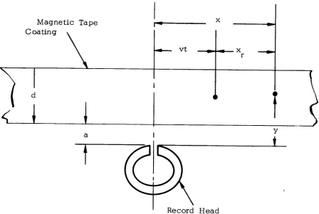
Figure 1 shows the dimensions used i n the formula given below. The d i s t a n c e above t h e record head t o ' t h e point a t which the magnetization is computed is Y and t h e distance along the t a p e axis from the record head center line to t h i s point is X

on tape t h a t is above the record head center line a t t = 0.

This is t h e axial d i s t a n c e to that point from the point Thus

xr

=

x + v t

(1)

where v is tape velocity and t is time. field in t h e X direction is

Hx.

The component of record head magnetic

The magnetization on tape is first computed using a non-interacting model, Demagnetizing effects are considered later, a s indicated below. The remanent magnetization on the tape is assumed to b e entirely in the longitudinal direction. The magnetization M, written a t the point (X, Y) on tape, is given a s a function by

Hx

by

I

Magnetic Tape 7

x -

Coating

vt -+ x_r

-0

1 d

Y

a I

Record Head

Fig. 1 Tape Recorder Coordinate System

Y

a I

t

I Record Head

[image:11.585.78.527.192.493.2]

c

AMPEX

where t is the point in t i m e a t which the point (X,

Y)

p a s s e s through the second head center plane and t 1 5 i

between s u c c e s s i v e bits.

the total number of non-zero values of M

[

H expressed in terms of X and t . by Eq. (1).

0

n a r e the points i n t i m e i’

In the l a s t term on

the

right of Eq. (21, n is (X, Y, t . ) ] and X is

X’ 1

In turn,

r 1

M o =

0

and

where

x

is the susceptibility of the magnetic material (see Fig. 2),

H I

is t h e threshold value of the magnetic field a t which switching c a n t a k e place and H is the saturating value of the magnetic field. In turn,

2

AMPEX

4

X

I

X"

2

/

AMPEX

if

i f

a nd

i f

A M - 0

(9)

The record head field longitudinal component is

where H (t) is the deep gap field and g is t h e gap width.

0

The deep-gap field, H (t) is a periodic function of t i m e , with

0

a period of twelve self-clocking bits.

of the pattern 0, 0, 1, 1, 1, 0 is shown i n Fig. 3.

interval of one bit, then for a pattern that contains a n odd number of ones (for example t h a t shown in Fig. 3 )

For example, H (t) for twelve b i t s N o t e t h a t if b is the t i m e

0

and for a pattern t h a t contains a n even number of ones

Next the alogarithm simultaneously t a k e s into account the effect of magnetic particle interaction, or demagnetization and computes the reproduce head flux.

average magnetization M given by

The first s t e p toward this objective is t o compute a n a

P a+d

where a is t h e head-to-tape spacing and d is the effective thickness of the magnetic material on tape.

*

Following this, we represent M by _a

n = I

AMPEX

0

I

7

0

no

I

I

I

l-4

l-4

l-4

0

-a)

E

d

l-4

I

I_

2

t

a

0

0

RR

67-

36

where

This Fourier series representation is p o s s i b l e b e c a u s e M 1 2 xb by Eq. (2) through Eq. (14).

and certain other previous equations,

is periodic i n a

In addition, from Eq. ( 1 2 ) and (13),

i f t h e 6 bit code contains a n odd number of o n e s and

i f t h e 6-bit code contains a n e v e n number of ones. A s a result, M c o n t a i n s a

only even harmonics i f t h e 6-bit code c o n t a i n s a n e v e n number and M contains only

number of ones. a

1 Ma llinson is given by

odd harmonics i f t h e 6-bit code contains

h a s shown t h a t t h e flux in t h e reproduce

--I

of o n e s a n odd

head @(t)

(16)

J. C. Mallinson, "Demagnetization Theory for Longitudinal Recording, I '

AMPEX

In E q s . (17) a n d (18)

where g is t h e reproduce head gap width, r

The output voltage from the reproduce head i, iven in terms of t h e flux by

where N is t h e number of turns on the reproduce head. and (20)

From E q s . ( l ) , (16)

The reproduce head output voltage is computed by Eq. (21).

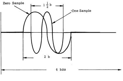
2. 1. 4 Computation of Sample Signals a n d Cross-Correlation Functions To compute a zero sample, we first find the output voltage from the reproduce head for a signal input t o t h e record head t h a t c o n s i s t s of six zero bits. Since for t h i s pattern

Ho

(t

+

B) = -H (t)

0

From Eq. ( 2 2 ) , we s e e t h a t t h e r e must b e a t i m e t a t which V is zero, and t h a t

0 r

V (t

+

mb) = 0 ( 2 3 )

r o

where m is a n y integer. T o construct the zero sample, S (t) we l e t

0

From E q s . (23) a n d (24)

Y;;(.t)

=

L,

(t.f

2 L

)

=-

0

and from t h i s a n d Eq. (25), we see that S 1s ccntinl:ocs c?t

3 0

a s shown in Fig. 4 .

AMPEX

-I

2 b

RR 6 7 - 3 6

6 bits

Fig. 4 S a m p l e Signals

[image:20.581.70.490.168.445.2]

T o compute a one sample, we first find t h e output voltage from the reproduce head for a signal input to the record head that c o n s i s t s of

six one bits. Since for t h i s pattern

From Eq. (26) there must b e a t i m e t a t which V is zero, and that

1 r

where m is any integer. T o construct the one sample, S (t) we let 1

( 2 8)

From Eqs. (27) and (28)

and from t h i s a n d Eq. (29), we see t h a t S is continuous a t t : r r ) ( ! C L I- 3/2b.

1 1

The cross-correlation function of t h e signal wiiii res:-,'ct to t h e

( T ! a c \_riven

z e r o sample, C

in t h i s application by

( 7 ) and with r e s p e c t to t h e one sample C;

AMPEX

J t = t o

+=

t ,

where X(t) is the signal. In t h e computer program, the integrals in E q s . (30) and (31) a r e computed using the trapezoidal rule.

Note that t and t a r e e a c h chosen from a multiplicity of values.

0 1

Furthermore, from E q s . (30) and (31) the phase relationship between C ( 7 ) and C1 ( 7 ) changes if

0

- t

0

is changed a s a r e s u l t

of

a new selection of t

or

t

or

both.

h a s a provision to keep this phase relationship from changing, and t o

insure t h a t So(t) and S 1 (t) a r e orthogonal. After

S

(t) and S,(t) a r e computed b y Eqs. (26) through (29), S (t) is slid along the t i m e a x i s so that its f i r s t a t a b s o l u t e maximum occurs a t the same value of t a s the f i r s t absolute maximum of So(t).

The program

1 0

.

0

1

Then

S

(t) and S,(t) have the t i m e relationship shown i n Fig. 3.

0

We define t h e "detectability", 6 ( ~ ) t o be

and compute

6 ( ~ )

from T = 0 to T = 6b. computed using the following algorithm:

Then t h e detector performance is

1. L e t T = 0 2,

0

For i = 1, 2

,...

6 find T . s u c h t h a t

1

3. L e t S

+

b e t h e set of integers i for which

a n d S

-

be t h e set of integers i for which

Then compute P a n d Q from

AMPEX

Another parameter required for the error rate compilations is p, defined a s

and computed b y t h i s equation. computed and printed o u t

Finally, t h e ratio P/p and Q/p are

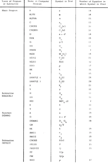
2. 1. 5 Comparison of Variable Names in Text and Computer Program

Table2.2 shows t h e variable names in t h e computer program opposite t h e corresponding symbols

from

the text.

2. 2 Description of the Computer Error-Rate Calculation (JPL-6)

2. 2. 1 General Description

This deck is used to compute error r a t e s in digital detection. error rate is computed on the basis of the d e t e c t e d zero and one s i g n a l P a n d Q, (computed in JPL-4 B), the noise power per unit bandwidth, N and the parameter

&

defined by

The

0’

where a is t h e head-to-tape spacing, and p(a) is the probability that the head-to-tape spacing will have t h e value 88a8’.

Table 2. 2 Comparison of Varible Names in Text and i n Computer Program JPL-4B

Yaame of Progrdni o r S u b r o u t i n e

M a i n Progrdm

S u b r o u t i n e MAGCAL3

Fu n c ti o n DEMAG

S u b r o u t i n e

DETECT

Ndrnc i n C o m p u t e r I'roqrarn A ALP1 I ALPHA C CROSS CROSS1 D

D FA

G H 0 HMIN RESX R C S Y Z RESX3 R I I O RK

R

SAMPLE U

SAMPLE 1

X Y H If 0 RES X Y A D DEMAG GR R K RMU 1 RMU2 CROSS PPLUS I'M I N US PP I'M RHO

S v m b o l in T r x t Numbcx of E q u a t i o n i n which S y m b o l is U s e d

14

3 4

1 s

1 5

3 0

[image:25.584.134.495.139.690.2]

AMPEX

2. 2. 2 Input

-

o u t p u t

Table 2.3 shows L e format of t h e d a t a cards used for t h i s program. The deep-in-gap magnetic field and the number of b i t s per inch (both which are input) are not used in the computation but appear in the printed output a s a n a i d to identification of t h e computed error r a t e values t h a t a r e printed out.

For e a c h error rate computation, the computer prints out, on a single line, the v a l u e s of

8,

No,

H

program prints out the values of N

8,

A (head-to-tape spacing), P/p, and

Q/p, in t h e order in which they a r e read in. T o permit the computation of a number of error rates, the program returns to read data card No. 4 (in Table 2.3) a t the completion of e a c h computation.

the b i t s per inch, and finally, the error rate. The

0'

0'

2. 2. 3 Error Function Complement

The algorithm for error r a t e computation employ the computation of t h e error function complement.

in t h e subroutine named ERROR Abramowitz and Stegun,

paragraph 7. 1. 26

of

t h i s reference

is used; otherwise, the algorithm of

paragraph 7. 1. 23 is used.

The error function complement is computed This subroutine u s e s algorithms, provided by If the argument e x c e e d s 2. 5, the algorithm of

2. 2. 4 Computation of Error Rate

The quantity ER(a) is computed by

where t h e ratios P/p and Q / p were computed by means of the program deck JPL-4B. Note that ER(a) is a function of a b e c a u s e P and Q are functions of a. Finally, t h e error rate, ER is computed by

1

Milton Abramowitz and Irene A. Stegun "Handbook of Mathematical Functions, ' I National Bureau of Standards, Applied Mathematics, Series No. 55, June 1 9 6 4 Pp. 298-299.

where p(a) is given b y Eq. (38), E R ( a ) is given b y Eq. (39) and al is t h e head-to-tape spacing beyond which errors occur e v e n in the a b s e n c e of noise.

n o i s e will c a u s e error, and the second term on t h e right of t h i s equation is the probability t h a t error will r e s u l t only from excessive head-to-tape

spacing.

the trapezoidal rule.

The first t e r m on t h e right of Eq. (40) is t h e probability t h a t

This integration is carried out in t h e computer program by u s e of

2. 2. 5 Comparison of Variable N a m e s in Text and i n Computer Program (JPL-6)

Table 2.4 g i v e s the names u s e d in computer program JPL-6 for the variables u s e d in t h e above d i s c u s s i o n of t h e error r a t e computation.

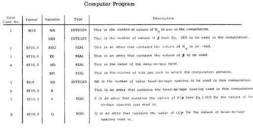
Table 2. 3 Data Card Description for JPL-6 Computer Program

D a t a

C a r d No. Format

8110

8F10. 0

8 F 1 0 . 0

8F10. 0

8110

8 F 1 0 . 0

8F10. 0

8 F 10. 0

V a r i a b l e

N N NEX RNO M HO BPI NA A P 0 INTEGER INTEGER REAL REAL REAL REAL INTEGER REAL REAL

D e s c r i p t i o n

T h i s is t h e n u m b e r of v d l u c s of N to u s e in t h e c o m p u t a t i o n .

T h i s is t h c n u m h e r o f v a l u e s i f ( s a c C q . 3 8 ) ) to h e u s e d i n t h e c o m p u t a t i o n . T h i s is an array t h a t c o n t a i n s t h c v d l u o s of N o to b e ! ( s e d .

T h i s i s a n a r r a y t h a t c o n t a i n s t h c v a l u e s of p to b e u s e d . T h i s is t h e v a l u e of t h e d e e p - i n - q d p f i e l d .

T h i s is t h e n u m b e r of b l t s p e r Lnch t o w h t c h t h e c o m p u t a t i o n p e r t a i n s .

NA i s t h e n u m b e r of v a l u e h e a d - t o - t a p c s p a c i n q t o be u s e d i n t h i s c o r n p u t a t t o n . T h i s i s a n a r r a y t h a t c o n t a i n s t h e h e a d - t o - t a p e s p a c i n g u s e d i n t h i s c o m p u t a t l o n .

P is a n array t h a t c o n t a i n s t h e ValllCS of P/p (see Eq. ( 3 9 ) ) for t h e v a l u e s o f hcd(.

t o - t a p e s p a c i n q l u s t r e a d i n .

[image:27.580.60.574.454.726.2]

AMPEX

.

Table 2. 4 Comparison of Variable N a m e s in Text and

i n Computer Program JPL6

I

Name i n Computer Program Symbol i n Text

A ERFCP ERFCQ

Ex

P PA PROD

Q

RNO

SUM

0 4

0

N I ER

3. 0 PRE-DETECTION STUDIES

3. 1 Absolute Output Voltage Multiplier

With the sole exception of program

JPL-2,

the original Fourier transform deck, all the computer outputs a r e now s u b j e c t t o t h e s a m e calibration factor on voltage.

If the number of _{turns on the reproduce head is N and the maximum.} tape remanence is 4nM g a u s s and the track width is umils and the t a p e

=locity is V ips, then the correct output voltage is derived b y multiplying the computer output by the factor;

r

For

example if; N = 250 turns, 4 n M r = 1000 g a u s s 0 = 80 m i € s

and V = 60 i p s (these typical figures being close to IBM compatible practice),

-

(''true -

("talc

6. 2 5 -

.

250

.

1000

.

80

.

60 or

-3

- x 7. 5 10 v o l t s ("true - ("calc

Since ( d c a l c is approximately 1 unit, we have (cItrue -

-

7. 5 milli-volts for t h i s example.

~

AMPEX

26

0

CI)

+

+

w

0

.+

0

0

+

a

0

N

I

AMPEX

As

another example, let u s consider an a u d i o recorder of t h e type u s e d i n t h e calculation of the noise power figures? Here we will typically have; N = 1000 turns, 4sMr = 1250 g a u s s ,

u

= 50 m i l s , V = 1 0 ips, which

-4

yields a conversion factor of 4. 10

.

The t a p e background noise l e v e l of

2 -1 1 - 4 2 2

u n i t s /cycle thus becomes 10 ( 4 . 1 0 ) volts /cycle which 2

e q u a l s 160 (nanovolts) /cycle.

Finally, it must b e remembered that none of t h e programs include a n y allowance for t h e well-known flux "shunting" effects in reproduce heads.

the output coil to total t a p e flux) are approximately 20 to 40%, the computer outputs m a y be anticipated to be proportionately high.

S i n c e typical head e f f i c i e n c i e s (i. e., t h e r a t i o of flux threading

3. 2 Comparison of the Fourier Series Program Output Voltage with Experiment

A test w a s made of the a b i l i t y of t h e six b i t program (Fourier Series) to d u p l i c a t e pulse crowding

or

bit interaction effects correctly. Typical r e s u l t s a t 3 2 00

BPI

a r e shown i n Fig. 5,

output v o l t a g e for t h e six b i t

NRZ

work 111000 is plotted a g a i n s t t a p e where t h e reproduce head

longitudinal d i s t a n c e for three v a l u e s of the d e e p g a p record field (Ho = 1500, 2250 a n d 3000 oe).

which correspond c l o s e l y with t h e a c t u a l case shown dotted, are: Other parameters in t h e calculations,

h e a d to t a p e spacing t a p e coating t h i c k n e s s record g a p length reproduce g a p length range of switching f i e l d s permeabilities

a = 20 d = 400 p "

= 500 p "

grec 'reprod

H1/H2 = lOO/SOO oe

= 250 p."

P1/P2 = 5/2

*See s e c t i o n 4.

It will be observed t h a t a l l the e s s e n t i a l features of the a c t u a l A s m a l l discrepancy is apparent signal are reproduced by the computer.

in t h a t the 2. 0 X SAT computer curve matches t h e actual curve better than the 1. 5 X SAT curve which should show the b e s t match.

in f a c t slightly underestimating pulse crowding.

2000, pulse crowding is due simply to the superpositim of a d j a c e n t pulses. A t BPI greater than 2000

the interference of the record zones, occurs. Such crowding is

,

of course, non-linear and non-super-imposable, and is dependent critically upon the record gap length, record deep g a p field and the specific record head field function being used.

to the use of the Karlquist head field expressions.

The computer is A t BPI less than about

a s is t h e c a s e here, additional pulse crowding, due to

The present computation error is most probably due

N o additional work upon the problem will be performed during the present contract. It m a y b e safely concluded t h a t no worse match than t h a t shown will occur, for any bit pattern, providing the BPI < 3000 for the 400 p " thick media or BPI < 6000 for t h e 200 p " media.

A more exhaustive program of experimental validation w a s under- taken a s a n extension t o the work reported here.

in Appendix 11. Suffice it to s a y that, upon such close examination, t h e program was found to be useable to higher b i t d e n s i t i e s than indicated above. In the saturation record level c a s e , the program is good to a t l e a s t 5, 000 BPI; a t lower record levels, (which would b e used) good agreements a r e found t o be a t l e a s t 10, 0 0 0 BPI,

3. 3 The Effect of Record Current Finite Rise T i m e s

A test w a s made of the effect of non-zero record current (or more pertinently record field) r i s e t i m e s .

the r e a s o n that the a c t u a l experimental waveforms, taken a t a tape speed of 7 5 IPS, used a waveform generator with 0. 5 p sec r i s e time.

d i s t a n c e along the tape is thus 37 p'l, to which may be added perhaps another 3 0 p " due to the limited frequency response (eddy currents) of the record head structure. The total rise distance of the record field is then probably about 7 0 p " , which is a n appreciable fraction of the bit length a t 3200 BPI (315 p"). It was felt to be worthwhile to e s t a b l i s h t h a t the r i s e t i m e effect w a s not contributing to the discrepancies observed.

This investigation w a s made for

The r i s e

The Fourier Series program was modified to permit exponential behaviour of d e e p g a p field (see Fig. 6 below).

Fig. 6 Exponential Behavior of Deep Gap Field

[image:34.590.60.525.431.637.2]

The factor x is simply t h e exponential t i m e c o n s t a n t multiplied Because mathematical complications a r i s e if the rise

0

b y t h e tape velocity.

distance is long compared to t h e bit interval, t h e program is restricted to x 1/2 X BPI. Figure 7 shows two waveforms produced for t h e six b i t word (NRZ)

-

111000 a t a d e e p g a p field H

distances, 0 and 156 p " .

a t 3 2 0 0 BPI.

.

0

of 1500 oe with two r i s e

0

The l a t t e r d i s t a n c e is one-half t h e b i t intervaf

It will be observed that, apart from a phase shift, wherein t h e f i n i t e rise d i s t a n c e c a s e is moved upstream on t h e t a p e with r e s p e c t t o the zero rise d i s t a n c e c a s e , there is indeed very little effect. It is concluded, then, that providing the rise d i s t a n c e s are not sufficiently long to c a u s e s e v e r e "staircasing" (i. e . , incomplete switching) of t h e record field, t h e effects are negligible.

This conclusion is not surprising, in view of our previous finding t h a t the i s o l a t e d pulse output waveform w a s virtually independent of t h e precise (saturation) recording conditions.

(i. e . , demagnetizes) and r e t a i n s little information a t wavelengths l e s s than t h e coating thickness.

nothing useful c a n be gained b y a n y of the more or less elaborate s c h e m e s of pre-shaping t h e input record current.

The written transition r e l a x e s

AMPEX

t

1

1,

I

t

5

0

0

+

+

I

I

2

po

3

N

0

0

OD

d

RR

67

-36

3. 4 Output Anomalies

In t h e course of a s e r i e s of over 100 runs investigating the peak- to-peak output voltage of a n "all ones" pattern on a function of d e e p g a p field

(H

1,

BPI and head-to-tape spacing, it w a s found, whenever the record head-to-tape spacing w a s comparable with the b i t interval being used, and whenever the record-head field was below the level required t o saturate the tape

(8. e., 500 o e contour beyond the the back side of the tape), that the output voltage w a s a n oscillatory function of the deep-gap field.

0

(See Fig. 8 .)

This oscillatory behaviour w a s not foreseen; neither could any reference t o it be discovered in t h e literature.

that some mistake in t h e computer program w a s causing the effect, and

nearly ten days (and almost 2 0 computer runs) were spent examining a variety of possibilities. A slight computer program error w a s discovered (concerning the algebraic s i g n of t h e increments in remanent magnetization acquired by tape elements) b u t rectification of this fault did not s t o p the oscillations.

finally found, by hand claculation, that the oscillations occur a s a direct consequence of the noninteracting remanence loop model

[

see MTPR #1,

kq.

111.

during the t i m e (or distance) t h a t a tape element is passing through the critical range of field strengths (H

record head.

It w a s assumed, erroneously

It w a s

The phenomenon only occurs when several field reversals occur

and H ) on the downstream s i d e of t h e

1 2

It is not known, a t this t i m e , whether such oscillation really occurs in practical systems.

only under conditions where the output signal is already a t l e a s t 20 db (factor of ten) below the peak level possible. It may, therefore, have e a s i l y escaped observation.

the old hi-fi buff's technique of d. c. erasing tape with a "horse shoe" permanent magnet which is placed obliquely a g a i n s t the tape.

the tape experiences a large longitudinal field, followed by a smaller field in the opposite direction, and c a n thus b e left with zero remanence.

A point worth noting is t h a t it is predicted to occur

The whole phenomenon is c l o s e l y related to

AMPEX

c

P

0.

Record Head-to-Tape Spacing = 50 pin. Reproduce Head-to-Tape Spacing = 50 u i n . Coating Thickness = 2 0 0 pin.

Record G a p Length = 150 pin.

Reproduce G a p Length = 2 5 p i n . Tape Switching Fields = 100/500 o e Permeabilities = 4/2

S i x B i t Word

-

All O n e s NRZ(M).

Fig. 8 Output Voltage Versus Deep G a p Field

[image:38.588.45.518.151.490.2]

It is of interest t h a t if the non-interacting M -H model were to b e replaced by a n empirical model of remanence acquisition, the effect would

still persist.

r

It is concluded, then, t h a t t h e effect calculated m o s t probably It was would be found in practice but is not of any great consequence.

decided, therefore, to l e a v e the computer program unaltered.

3. 5 Modification of the Program to Correct the Depth of Recording

It will be recalled t h a t after e a c h lamina of tape h a s been recorded upon, t h e next s t e p in the computer program is the computation of the average

mag ne t i z a tion;

a

+

d '

M dy (See section 2. 1) 1

M = -

d ' sa

-

The points of concern here a r e the value of the upper l i m i t of integra- tion (a+d') and the effective tape thickness d ' to be used when the whole depth of t h e coating is not completely magnetized (i. e . , saturated).

Previously, this effective t a p e depth (d') h a s been calculated according to t h e smaller of

d ' = d

or a

+

d ' = depth of 100 oe contour on head center plane.

Thus any material which did not experience even the minimum switching field (100 oe) w a s merely ignored throughout the remainder of the calculation. This procedure obviously g i v e s the maximum reasonable value for d'.

minimum reasonable value would b e given by ignoring a l l material which is not saturated, i. e. :

AMPEX

d ' = d

or, a

-+

d ' = depth of 500 oe contour

It will b e appreciated that much of the remaining program is critically dependent (at low values of t h e deep-gap field

Ho)

on the

particular criterion chosen. This occurs mainly because the demagnetization and remagnetization processes a r e very s e n s i t i v e to the product k d ( or k d')

(see page 5, MTPR #3). pulse width

page 5, MTPR #3), because even a t H = 500 oe, the 100 oe contour still penetrates a 200 p " coating completely.

of pulse crowding a t low record currents,

The old criterion (100 oe contour depth) led to t h e being almost independent of deep-gap field (see Table

IV,

0

The r e s u l t is the over-estimation

Obviously no single correct criterion c a n be decided upon. This unfortunate situation is forced upon us by our desire to u s e the c l o s e d form solutions of t h e demag-remag problem.

iteration is believed to b e of virtually astronomical magnitude (200 x 200 calculations per bit cell per iteration).

The alternative procedure using

It h a s been decided to resolve t h i s problem by using a n "engineering" The effective depth shall b e considered to be half way

approximation.

between t h e maximum and minimum values possible; i. e., we t a k e d ' to be the smaller of

d ' = d

or a

+

d ' = depth of the 300 oe contour

It is noted, in passing, that Kostyshyn (IEEE Trans. Mag.

2

3, page 236, Sept. 1966) assumed the minimumreasonable depth. In other words, he ignores completely the partially magnetized material.

3. 6 Head t o Tape Spacing Effects

Previously, investigations have b e e n made (see MTPR #2 and 3) of t h e effects of varying t h e head-to-tape spacing on t h e amplitude (and 20% p u l s e width) of isolated transitions.

to t h e c a s e of repetitive transitions.

(NRZ) i. e.

,

t h e record current changes s i g n a f t e r e a c h b i t interval.

b e realized that, even though a n i s o l a t e d pulse is i n s e n s i t i v e to head-to- tape spacing b e c a u s e it is n o t rich i n harmonics of wavelength shorter t h a n the coating t h i c k n e s s , t h i s simple conclusion need not hold in t h e repetitive pulse case.

a n d only t h e high harmonics, which a r e very s e n s i t i v e to head-to-tape

spacing remain. Typical data is shown in Fig. 9 , in which figure is shown the output voltage, a t 8000 BPI, v e r s u s deep-gap field, for four cases;

Here we report similar d a t a applied The six-bit word c h o s e n is "all ones"

It will

Here all t h e low

[

<2/BPI] harmonics a r e forbidden

a) b) c) d)

record and reproduce spacing = 100 p "

record spacing = 1 0 0 pL1, reproduce spacing = 20 p"

record spacing = 20 p", reproduce spacing = 1 0 0 p "

record and reproduce spacing = 20 p "

2

The curves a r e labeled (a a ) where a is t h e record-head spacing and a

1' 2 1

is t h e reproduce-head spacing.

Several comments may b e made about t h e s e r e s u l t s ,

a) Any spacing greater t h a n t h e standard 20 p " a t either head c a u s e s

0'

losses which cannot b e recovered completely b y adjustments of H

b) Whenever the record head-to-tape spacing is large, s o m e recovery of signal is possible by increasing t h e record current (i. e . , Ho).

the (100, 20) and (100, 100) curves both peak a t Ho a n d (20,100) both peak a t

Ho

-

-

1 5 0 0 oe.

approximately 6 db, where a s t h e l o s s of s i g n a l due to 100 p " record-head spacing is approximately 10 db.

AMPEX

0.

‘P

0.

0.0 1

0

(100, 100)

101

4000 5000 6000

0 1000 2000

Head-Tape S p a c i n g as noted. 8000 BPI

d = 200 pin.

grecord = 150 pin.

11111 NRZ

oe

Fig, 9. Output Voltage Versus H a t Various Head Tape Spacings

0

c) Whenever the reproduce head-to-tape spacing is large, This signal loss is approximately a very large loss in signal occurs.

20 db regardless of the record current level.

a t 8000 BPI the output signal is almost purely sinusoidal, of wavelength 250p", and consequently the increase i n reproduce spacing loss is:

This is not unexpected, s i n c e

= 17. 5 db

-

- 55

[

100

-

201

55

[

(azl1

-

q2]

A 250

We conclude, therefore, that a t high b i t d e n s i t i e s t h e "uncompensated" record-head spacing loss is about one third the reproduce spacing loss.

If the record current is readjusted, the "compensated" record-head spacing loss need only be about one fifth the reproduce spacing loss.

spacing loss is c l o s e l y approximated by the usual 55 a/A type expression. The reproduce

3. 7 Pulse Crowding Graphs

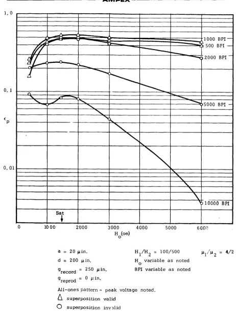
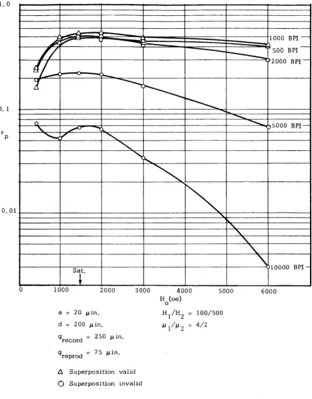
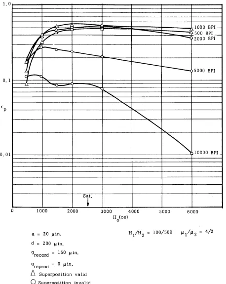
A s called for in t h e contract, sufficient computer runs have been

made t o derive graphs of output voltage v e r s u s b i t density.

graphs shows t h e computer peak output voltage (i. e . , not a d j u s t e d to yield absolute volts) v e r s u s d e e p g a p field for five b i t d e n s i t i e s , t h o s e corres- ponding to 500, 1000, 2000, 5000 and 10,000 BPI respectively. The data is shown in Figs. 10 through 13 each figure applying to a different pair of heads. In Fig. 1 0 , the record g a p is 250 p", t h e reproduce g a p zero, Fig. 11 250, 75 p", Fig 12, 150, 0, and Fig. 13, 150, 75p". The head-to-tape spacing on all runs w a s equal to 20 p " (the nominal contact value), the tape coating

thickness w a s 200 p", the range of switching f i e l d s l00/500 oe and permeabilities

4/2. An additional piece of information, included i n all the graphs, is whether

or not super-position (of output pulses) a p p l i e s or not.

a p p l i e s when t h e original recorded magnetization patterns a r e completely separate a n d distinct, and t h u s pulse crowding (or b i t interaction) only occurs during the (linearly super-imposable) demagnetization, remagnetization, f l u x

Each of t h e

AMPEX

0. 1

E

P

0 . 0 1

0 10 00 2000 3000 4000

Ho(oe)

5000 600C

H 1/H 2 = lOO/SOO p1’/p2 = 4/2

H v a r i a b l e a s noted

BPI v a r i a b l e as noted

0

a = 2 0 p i n . d = 200 p i n . grecord = pin-

!Jreprod = 0 p i n .

All-ones pattern

-

p e a k voltage noted. s u p e r p o s i t i o n valid

0

s u p e r p o s i t i o n i n n l i d

Fig. 10 Pulse Data Crowding

[image:44.588.52.514.59.668.2]

1. 0

3. 1

E

P

0 . 0 1

a = 2 0 p i n . d = 200 p i n . grecord = 2 5 0 p i n '

greprod = 7 5 p i n .

A Superposition valid

0 Superposition invalid

[image:45.581.89.544.81.661.2]

+

AMPEX

1 . 0

0. 1

E

P

0 . 0 1

0

I I I I

I I I 1

I

I

I

,

I

500 BPI- 2000 BPI

5000 BPI

7

*

+

1000 2000 3000 4000 5000 6000

Ho(oe)

a = 2 0 p i n . d = Z O O p i n . grecord = 150 p i n . greprod = 0 u i n .

0

Superposition invalid Superposition v a l i d

Fig. 1 2 Pulse Crowding Data

[image:46.580.48.506.87.662.2]

0 1000 2000 3000 4000 5000 6000

a = 2 0 p i n . H /H2 ₁ = lOO/SOO oe _p1/p2 = 412

d = 200 p i n . grecorci greprod

= 150 p i n .

= 7 5 p i n . s u p e r p o s i t i o n valid

0 s u p e r p o s i t i o n invalid

[image:47.580.74.527.94.667.2]

AMPEX

The following comments may be made.

a. In a l l c a s e s the effects of bit crowding do not become severe until above 2000 BPI.

yFe 0 tape, principally dependent upon the coating thickness used. If standard digital 400 PI' thick tape were t o b e sub-

stituted for the present 200 p " tape, the effects of crowding would then become severe above 1000 BPI.

Very little difference is to be noted a t deep g a p fields near the saturation level between the record gap equals 250 p " and

150 p " data. This is, of course not unexpected.

This "break point" is, with standard 2 3

b.

A t low bit densities, the output voltage is governed almost entirely by the demagnetization effects d i s c u s s e d in MTPR #l. The d e t a i l s of the recording process a r e e s s e n t i a l l y forgotten. A t high bit d e n s i t i e s the recording t a k e s place in a narrow zone

downstream of the record gap center line (trailing edge effect). The geometry of t h i s zone is not simply related to the record g a p length. It is a function of the d e e p gapfield, the depth into the tape, the tape particle switching fields, as well a s the g a p length.

The only region in which appreciable differences occur between

the two record gap lenghts is at very high record l e v e l s (greater than two t i m e s saturation) and very high BPI.

a t

Ho

= 6000 oe and a t 10, 000 BPI, the g

about a factor of three (10 db) lower than in the 150 pt' c a s e .

It will b e noticed that,

= 250 p'' data is record

We may conclude that smaller g a p lengths a r e better only in poorly designed regions of operation.

c.

As

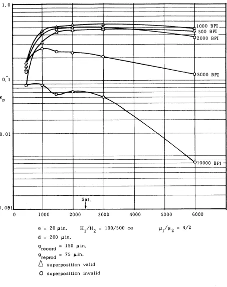
w a s mentioned i n MTRP #4, a t the higher BPI'S, it pays increasing dividends to operate below the saturation (i. e., self-erasing) level.

d. Super-position is valid for all the 500 and 1000 BPI data. A t 2000 BPI the 250

above 1500 oe d e e p g a p field.

is super-imposable a t 3000 oe d e e p g a p field.

record g a p data is n o t super-imposable The 150 y " record g a p d a t a

Above 2000 BPI neither head y i e l d s super-imposable r e s u l t s at a n y d e e p g a p field.

e. The effect of reproduce g a p is s e e n t o be very s l i g h t i n t h e

region investigated. The zero length g a p obviously will show no interference effects, t h e 75 y " case will have a null a t

X

= 75 y", corresponding to 26, 666 BPI and will show negligible g a p l o s s e s below A = 150 y " (i. e., 13,333 BPI).

borne out in t h e data where e v e n a t 10, 000 BPI there exists less than 2 db difference.

This is

A practical rule emerges concerning t h e s e l e c t i o n of reproduce g a p The g a p length should b e a s large a s possible but no larger t h a n lengths.

the smaller of: a.

AMPEX

3.

a

Peak Shift Calculation

In accordance with the contract, calculations of peak s h i f t have been made.

following conditions :

The computer recorded a s'ingle pair of transitions under t h e

Coating t h i c k n e s s d = 200 p "

Head-to-tape spacing Switching fields H1/H

a = 20 p,"

= l O O / S O O oe 2

Permeabilities p1/p2 = 4/2

a s noted

a s noted

0 0 1 1 0 0

NRZ

Record g a p Reproduce g a p D e e p Gap field B i t pattern

X

€ _I

' I

P

IAxr

\-

I

Percentage peak s h i f t equals 100 &/BPI

RR 67-36

Table 3. 1 Percentage Peak Shift a s a Function of BPI, Deep Gap Field, Record and Reproduce G a p s

BPI

2,000

5 , 0 0 0

10,000

0

H

'record = 150 = 75 'reproduce

0. 15 0. 5

1 1. 4 10. 0 14. 0 12. 6 37.7 43. 8

150 0

--

0. 65 0. 55 0. 9 9. 0 13. 5 7. 5 32. 5 39. 0

250 75

--

0. 75 1. 6 4. 0 12. 2 18. 8 23. 2 39. 1 142. 0

250 0

0. 25 0. 7 5 1. 75 2. 7 11. 0 17. 5 17. 1 34. 2 151. 0

Several, not unexpected, trends are evident: a.

b.

The percentage peak shift i n c r e a s e s with increasing BPI. The percentage peak s h i f t i n c r e a s e s with increasing d e e p g a p field.

The percentage peak s h i f t i n c r e a s e s with increasing record g a p field.

The percentage peak shift i n c r e a s e s with increasing reproduce g a p length.

c.

d.

The practical r u l e s which emerge are: a.

b.

Peak s h i f t is negligible below 2000 BPI.

In the neighborhood of 5000 BPI t h e u s e of saturation* record current l e a d s t o peak s h i f t s of order 10%

-

20%, t h e p r e c i s e value being dependent upon the g a p l e n g t h s used. The peak [image:51.587.82.501.92.356.2]

AMPEX

c. In the neighborhood of 10, 000 BPI the u s e of saturation* record currents l e a d s to large peak shifts (>30%).

of

two

t i m e s saturation currents c a u s e s over 100% peak shift. The situation may be largely corrected, however, by the combination of smaller record gaps (<150p") and lower record currents (about one-third of saturation).

The u s e

*Saturation means self erasing (H = 1500 oe for record g a p = 150 p "

(H = 2350 oe for record g a p = 250 p")

0

0

I

4 . 0 DETECTION OF SIGNALS OF KNOWN SHAPE IN THE PRESENCE OF WHITE

GAUSSIAN

NOISE

4 . 1 Signal Representation

4. 1. 1 Restrictions

W e consider only s i g n a l s of finite duration T and fi n i t e bandwidth W.

In t h i s c a s e the s i g n a l s(t) is completely described by a finite set of points.

4 . 1. 1 Sampling Theorem

Fourier integral: s (t) df

-OD

The signal is bandlimited; the spectrum can b e developed i n Fourier series: Complex Fourier coefficients

(C

*

: conjugate of C ):

n

n

-W

Comparing with t h e Fourier integral of s(t):

n

The spectrum is determined by t h e v a l u e s s(n T )

,

and from t h e spectrum t h e time-function s ( t ) can be computed. W e need only know sampled v a l u e s

7 =

-

1 s e c o n d s apart to reconstruct t h e complete s i g n a l . S i n c e t h e s i g n a l

2w

is of duration T , s(t) is given b y a s e t of T./T=

-

2WT could be represented by a point i n a 2\VTi'-dimensional s p a c e .

4.1.3 Ideal

Lowpass

We determine t h e impulse r e s p o n s e of a n i d e a l lowpass:

-W

4. 1. 4 Representation of s ( t ) s(t)

= E

s ( n 7 ) h (t

-

n r )

s i n 2 r W t

-

n d 2n ~ (

-

nT t ) =

C

s ( n r )

Total number of points: 2WT s i n n (2wt-n) 2WT

s(t) =

c

s-

1 2w

r =

-

(4. 1) n (2Wt -n)

I1

n

=1

That t h i s r e p r e s e n t s t h e signal s ( t ) is readily seen:

-The constructed s i g n a l c o n s i t s t s of a superposition of impulse r e s p o n s e s from a lowpass filter of bandwidth W; h e n c e s(t) h a s a bandwidth W.

AMPEX

The functions q, =

sin

I7 (2Wt-n) constitute a s e t of Grthogonal functions:

g (2Wt-n)

Proof:

*) conjugate value

1 := H(f) e 1217 f n r

for n = m ,

This is

-

1 ₀ else.

2w

4.1.

5 Integration of Signals

s

(t);

s

(t) a r e two s i g n a l s with same restrictions a s s t a t e d i n 1.1.

0 1

5

So(t) sl(t) dt

+Q

=!(E.

n on s n ) ( i s l m qm) dt (see (4.1))

-W

-0)

applying t h e orthogonality (2):

.

2 w T

= 1

[L

4,

i f so, y a r e v e c t o r s

2W

-

i n t h e 2WT dimensional s p a c e :

4 . 2 Signal Detection

4. 2. 1 Distortion of a Signal by White G a u s s i a n Noise n(t)

. 2

n

- -

c)

; s p e c t r a l d e n s i t y Gn(f) =

No

2 0

e

p(n) =

-

1

( 4 . 3 )

In t h e system s i g n a l a n d n o i s e a r e a s s u m e d t o h a v e t h e

same bandwidth

3 -

W: mean n o i s e power n

-2

, 2

n equals t h e v a r i a n c e 0

.

S i n c e we h a v e w h i t e n o i s e , n i s s t a t i s t i c a l l y independent a t different p o i n t s i n t i m e . The probability of a c e r t a i n deformation x(t) of s(t) is e a s i l y

computed:

-

No*

W.

original signal d i s t o r t e d s i g n a l

x - s

i i

1,

then t h e probability If x(t) is r e p r e s e n t e d b y t h e vector

-

x =

[x

1 ' X2'

...x

2 w T

AMPEX

The joint probability is t h e product

of

the individual probabilities. This holds for white g a u s s i a n n o i s e .

'

4 . 2 .

2

Likelihood

Test

Given a n observation x(t) w e have

to d e c i d e which signal

s

(t) of a qiven k

alphabet is t h e most l i k e l y one. Emitting

a

signal s k ( t ) , t h e probability

of

receiving x(t) is proportional t o

Assuming t h a t e a c h

s

(t) is equally likely emitted, w e have

to c h o o s e that

sk, which g i v e s t h e maximum p (51 s )

.

Taking t h e logarithm of (4):

k

k

2

+ -

0 0

2 1 2

2N W F S k i

?(Xi

-

Ski) =

c

-

-

1

2N W 'Xiski

C'

-

-

2 N W 1

0

C is a c o n s t a n t , independent of index

k.

Applying equation (3):

Interpretation:

k

\s;(t) dt = Energy E of a l p h a b e t s i g n a l s

k

Sx(t) sk(t) dt = Peak output of a correlator or m t c h e d filter.

Decision criterion:

(4.5)

4. 2. 3 Error Probability; k = 2

We h a v e to c h o o s e between two s i g n a l s s (t), s (t)

.

To find t h e maximum

0 1

(4. 5) we may consider the difference of t h e

two

e x p r e s s i o n s

1

i o

N

'u

=

\

x(t) (s -s ) d t

- -

(E1 - E )

0 0

NO

1

Decision:

u

> O

: s

x(t) c a n b e

W e make a false d e c i s i o n if:

1)

x

and u

'40

2)

xo

a n d u

> O

1

Both

cases

a r e completely symmetric; i t s u f f i c e s to study one. (The c h a n c e of having o n e of the two

cases

is

SO%,

b e c a u s e

s

to

be equally likely).

s

h a s been assumed

0 , 1

W e s e a r c h for the probability

of

having

x

and u

<

0

1

1

(sl

+

n)

(s

- s

) d t

- -

(E1

-

Eo),

t

o

N

0 0

N

with

A S = S

- S

1 0

A E = E 1 - E 0

1 AE

F

(sli

+

nil

b.si

-

N

N W 0

u =

0

W e know t h e probability d e n s i t y function of t h e n.:p (n,); w e h a v e to find

i n i

u is

a

l i n e a r combination of t h e random variable n * l i k e n u w i l l therefore

have g a u s s i a n distribution. Mean and variance for u have t o be calculated: in i '

AE

As(t) d t

- -

N

0 0

N

-

-

1

Z S

A s i - - - -

AE

0

N W i li N

u =

0

-

2 2

- -

-

i i 1 j i j

(u

- E

) 2

=(@r

L

As. n

,

b e c a u s e n . n = n n = 0

-

2

i 0

n = N * W

2

2 2

u = -

C A S = l - s l ~ s (t) d t and

0

N

u

N W i

0

1 - 2

. 2 0

--2 (u ' U )

e U

1

P(U) =

Th e error probability is:

1

ER

= _{p(u) du =}

-

3 U du

2

Defining erk(8) =

-

e dx we find

u

ER

= erfc(P) ; /3=

- -

u n

-

AE

1 N

s

A s

dt

- -

-

s

A,

s 2 ( t ) d t

0

N

0 0

N

2.

u

=

u

2

$

A

s 2 ( t ) dt N

0

(4. 6)

.

AMPEX

0

p=

-

F-

N

Using (3):

p=

- -

1 I

which

c a n b e interpreted

as'

follows:

(4. 7)

-

rNoW = n : rms v a l u e of n o i s e

E s 2 = "length"

of

the d i s t a n c e vector

- -

s

-

s

i n t h e 2WT-dimensional s p a c e

1 0

Defining

I

clr

e

1

and

I

he

I

a s t h e peak amplitudes for

x

= s,, and

x

= s respectively

0

1 0

er@ =

1

s

--

-w

- 2 dx

e

- X

I

I

and]Ae

I

c a n b e computed from t h e correlation functions:

1 0

(4. 8)

x (t)

,

x (t) a r e t h e a c t u a l l y r e c e i v e d s i g n a l s for a " 0 " and

a

"1"

0 1

r e s p e c t i v e l y .

4. 3 Concerning Dropouts: Conclusions and Plan of A c t i o n

(a) The differences i n drop-out behavior are sufficiently g r e a t between different reels of t a p e to preclude a n y meaningful statistical a n a l y s i s . This comment a p p l i e s even if one r e s t r i c t s t e s t i n g to s a m p l e s of o n e manufacturer, or indeed, to s a m p l e s slit from t h e s a m e original doff.

(b) The drop-out count on a n y one r e e l of t a p e is extremely dependent upon the method of testing. Track width, head contours, t a p e t e n s i o n , tape speed are all factors which c a n a l t e r t h e drop-out count b y several orders of magnitude.

AMPEX

locations and can, upon microscopic examination, b e a s s o c i a t e d with physical defects. The number and position of s u c h d e f e c t s change only slowly with repeated passes of t h e tape. It is, therefore, reasonable to a s s u m e , i n t h e computer-simulation of drop-out behavior, that the head-to-tape spacing is perturbed equally during both the record and reproduce cycles.

(d) In fact, there is no physical distinction between drop-outs and the so-called surface noise. The complete n o i s e spectrum of tape shows broad-band, almost white noise to which is added, a t low

frequencies, surface noise. A drop-out is nothing more

or

less than a n i n s t a n c e of t h e surface n o i s e exceeding some arbitrary level and/or duration.

For the purpose of computation, however, it is a great s i m p l i - fication to a s s u m e t h a t t h e drop-outs are long in duration compared to t h e six b i t word. This means that the head to tape spacing may b e considered to be c o n s t a n t during the whole six bit word calculation. This simplification which will b e adopted for the remainder of this programe is shown below

Assumed Surface

Noise

NO Actual Surface Noise "White" Noise

0

'f

1 6 x BPI

(e) Similarly, while there is no a priori physical justification for assuming that a drop-out extends uniformly across the whole track width, such will b e assumed in the computer program. This is, of course, a considerably m o r e restrictive assumption than t h a t i n (d) above.

Intuitively one expects t h e longitudinal and transverse dimensions of a drop-out to b e comparable. What we a r e r e a l l y presuming here is t h a t a n effective head-to-tape spacing exists, in which t h e tape and head planes are exactly parallel for dimensions greater than the track width. The validity of t h i s approximation will shortly b e t e s t e d (see below).

(f) W e s e e k a typical probability d e n s i t y versus effective head to tape spacing curve.

AMPEX

I

Purely i n the i n t e r e s t s of simpl