Micro-scale Observation.
Thesis by
Krzysztof Chalupka
In Partial Fulfillment of the Requirements for the Degree of
Doctor of Philosophy
California Institute of Technology Pasadena, California
2017
Acknowledgements
From my mother Barbara I learned to always push myself to the limits, and about honesty and decency. From my Polish friends Artur, Filip, Jagoda, Kuba, Marek, Ula, Wojtek, Zuza, that camaraderie tran-scends time and space.
From Master Ian Cameron of Edinburgh that training is its own reward, and so is mastery; and that the only thing that always goes with the flow is the dead fish; a set of exercises that saved my heart and stomach; to appreciate depth of character and resolution; and about music creative yet unpretentious.
From the I Ching, to seek out the subtleties of reality without resort to pompous spirituality. From Kun Zhang, to carefully remove snails into safety from the walkway during rainy nights. From my Chinese family, that family can and should be at the center of one’s life; and to be generous. From Alex, to think about the other’s mind before approaching them. From Aram, to fight against a larger and stronger opponent. From Bo, that cross-cultural friendship can be European. From Ron, I learned that there are people whose problem-solving skills far surpass mine. From Steve, I received an education in American friendship and how to respect it. From Tristan, I learned integrity and liberty.
From professor Yisong Yue, to mellow down (and not to write angry peer reviews).
From professor Doris Tsao, a passion for science, and a single-minded determination to reach a goal; that nothing is true by default, but only after I understand myself why it should be so.
From professor Frederick Eberhardt, to distrust any idea, thought or assumption, especially my own, until it is analyzed and broken into pieces and rebuilt in my own mind many times over.
From professor Pietro Perona, I learned to believe that there are still pioneers in science, and to will to be one of them; to be patient and kind to those without my experience or knowledge; to think clearly, and in terms of principles, goals, and people.
Abstract
This book introduces new concepts at the intersection of machine learning, causal inference and philoso-phy of science: the macrovariable cause and effect. Methods for learning such from microvariable data are introduced. The learning process proposes a minimal number of guided experiments that recover the macrovariable cause from observational data.
Mathematical definitions of a micro- and macro- scale manipulation, an observational and causal partition, and a subsidiary variable are given. These concepts provide a link to previous work in causal inference and machine learning.
The main theoretical result is the Causal Coarsening Theorem, a new insight into the measure-theoretic structure of probability spaces and structural equation models. The theorem provides grounds for automatic causal hypothesis formation from data. Other results concern the minimality and sufficiency of representa-tions created in accordance with the theorem.
Contents
Acknowledgements iv
Abstract v
1 Introduction 6
1.1 Causal Feature Learning . . . 6
1.2 Macrovariables in Science . . . 7
1.2.1 Ambiguous Manipulation and Causal Macrovariables . . . 8
1.2.2 Macrovariables Are Task-Specific . . . 9
1.3 Example Microvariable Cause-Effect Systems . . . 10
1.3.1 Images and a Spiking Neuron . . . 11
1.3.2 Hue and Skin Conductance . . . 13
1.3.3 Images and Neural Populations . . . 14
1.4 Related Work . . . 17
1.4.1 Computational Mechanics . . . 17
1.4.2 Causal Graphical Models . . . 17
1.4.3 Machine Learning and Artificial Intelligence . . . 18
2 Supervised Causal Feature Learning 20 2.1 Advances in This Chapter . . . 20
2.2 Theory . . . 21
2.2.1 Visual Causes as Macro-variables . . . 21
2.2.2 From Micro- to Macro-variables . . . 22
2.2.3 The Causal Coarsening Theorem . . . 24
2.2.4 Set-up and Definitions . . . 24
2.2.5 The Complete Macro-variable Description Theorem . . . 27
2.2.6 Predictive Non-causal Information in the Macro-variable Cause . . . 28
2.3 Algorithms . . . 29
2.4 Experiments . . . 30
2.5 Proofs . . . 30
2.6 Additional Acknowledgement . . . 34
3 Unsupervised Causal Feature Learning 35 3.1 Advances in This Chapter . . . 35
3.2 Theory . . . 36
3.2.1 Learning the Causal Hypothesis . . . 36
3.2.2 Weeding Out the Spurious Correlates . . . 38
3.2.3 Subsidiary Variables and the Sufficient Causal Description Theorem . . . 40
3.3 Algorithms . . . 43
3.3.1 Choosing the Number of States . . . 43
3.4 Experiments . . . 46
3.5 Proofs . . . 48
4 Learning Optimal Interventions 53 4.1 Advances in This Chapter . . . 53
4.2 Theory . . . 53
4.3 Algorithms . . . 54
4.4 Experiments . . . 55
4.4.1 The GRATING Experiment . . . 56
4.4.2 The MNIST ON MTURK Experiment . . . 56
5 Application to Climate Science 61 5.1 Advances in This Chapter . . . 62
5.2 El Ni˜no–Southern Oscillation . . . 62
5.3 Experiment: Learning Pacific Macro-variables . . . 63
5.3.1 Dataset . . . 64
5.3.2 Pacific Macro-Variables . . . 65
5.3.3 Varying the Number of States . . . 67
5.3.4 Reshuffled Data . . . 69
5.3.5 Challenges to Establishing Causality . . . 69
6 Causation without Intervention 71 6.1 Advances in This Chapter . . . 71
6.2 Related Work . . . 72
6.2.1 Additive Noise Models . . . 72
6.2.3 Desiderata . . . 73
6.3 Assumptions . . . 73
6.4 An Analytical Solution: Causal Direction . . . 74
6.4.1 Optimal Classifier for BinaryXandY . . . 74
6.4.2 Optimal Classifier for ArbitraryXandY . . . 76
6.4.3 Robustness: Changing the HyperpriorF. . . 77
6.5 A Black-box Solution: Detecting Confounding . . . 80
6.6 A Black-Box Solution to the General Problem . . . 81
6.7 Discussion . . . 83
6.8 Conjectured Application to Causal Feature Learning (CFL) . . . 84
7 Discussion 86 7.1 CFL in the Real World: Assumptions and Challenges . . . 87
7.1.1 Discreteness of Macrovariables . . . 87
7.1.2 Smoothness Assumptions During Learning . . . 88
7.1.3 Why Not Naive Clustering? . . . 88
7.2 Open Problems . . . 90
7.2.1 Learning Without Experimentation . . . 90
7.2.2 Continuous Macrovariables . . . 90
7.2.3 Cyclic Microvariable Graphs . . . 90
List of Theorems
1 Definition (Observational Partition, Observational Class) . . . 22
2 Definition (Visual Manipulation) . . . 23
3 Definition (Causal Partition, Causal Class) . . . 23
4 Definition (Visual Cause) . . . 23
5 Definition (partitionΠf(I)) . . . 24
6 Theorem (Causal Coarsening Theorem) . . . 25
7 Definition (Spurious Correlate) . . . 27
8 Theorem (Complete Macro-variable Description) . . . 27
9 Definition (Causal Intervention on Macro-variables) . . . 28
10 Lemma . . . 30
11 Definition (Unsupervised Observational Partition, Unsupervised Observational Class) . . . . 36
12 Definition (Microvariable Manipulation) . . . 38
13 Definition (Unsupervised Causal Partition, Causal Class) . . . 39
14 Definition (Macrovariable Cause and Effect) . . . 39
15 Definition (Macrovariable Manipulation) . . . 40
16 Theorem (Unsupervised Causal Coarsening Theorem) . . . 40
17 Definition (Subsidiary Causal Variables) . . . 40
18 Theorem (Unsupervised Sufficient Causal Description) . . . 42
19 Definition (Partition Product, Macro-Variable Composition) . . . 42
20 Definition (Non-Interacting Subsidiary Variables) . . . 42
21 Definition (Manipulator Function) . . . 53
22 Definition (Precision) . . . 66
Acronyms
Chapter 1
Introduction
During my time at Caltech, I developed — together with Pietro Perona and Frederick Eberhardt — the theory and algorithms that aim at solving a previously open problem in machine learning and causal inference. Concisely stated, the problem is as follows. Learn, by looking at low-level measurements, a maximally compressed representation of the causal mechanisms underlying these measurements. Part of this book is dedicated to defining the mathematical apparatus necessary to approach this question. This leads to the first algorithms solving the task, both in settings with and without supervision. The algorithms extract features of the data that are, in a well-defined sense, causal features: changing the underlying data has an effect on a system of interest only inasmuch as the value of the causal features changes. Hence the name of the framework, CFL.
Much of this book contains results and in some cases text passages from four peer-reviewed publications I am a co-author of (Chalupka et al., 2015, 2016b,a,c). Chapter 6 contains new material available online but not peer-reviewed (Chalupka et al., 2016d). Computer programs that implement our algorithms and reproduce some of the experimental results presented in this book is available online athttp://vision.caltech. edu/˜kchalupk/code.html.
1.1
Causal Feature Learning
CFL is a machine learning and causal inference framework with two goals: 1. Formation of high-level causal hypotheses using low-level input data, and 2. Efficient testing of these hypotheses.
col-Figure 1.1:Causal Macrovariables. Macrovariables in science are functions of the underlying microvariable space. Each such functionf corresponds to apartition on the microvariable state space, defined by the equivalence relationx1 ∼x2 ⇐⇒ f(x1) =f(x2). (A) Temperature may be defined as the mean kinetic
energy of a system of particles. It is a one-dimensional function of a high-dimensional system consisting of a large number of particles, each one with a mass and velocity. (B) El Ni˜no is defined as the sea surface temperature (SST) anomaly in a specific region of the Pacific Ocean exceeding 0.50C. It is a binary function of the high-dimensional sea surface temperature (SST) map. (C) Primate brains are thought to have areas specialized for face detection (see Tsao et al. (2006) for direct evidence in the macaque cortex). “Presence of a face” is a binary function on the space of all images.
lecting evidence from such experiments.
Steps (a) and (b) are guided by prior knowledge, intuition and formal reasoning. CFL aims to augment or fully automate this process in situations where observational data is plentiful, reducing the bias resulting from pre-conceived ideas of the scientist. The method is predicated on the idea that if the data in fact contains high-level features (such as female faces) that are causal, then these ought to be detectable by a learning algorithm. In addition, CFL distinguishes between features that are related by directcausationfrom features that are related through common causes. For example, atmospheric pressure causes the needle of the barometer the change, but the needle’s position is neither a cause nor an effect of rainfall, with which it nevertheless strongly correlates.
1.2
Macrovariables in Science
In CFL, the distinction between high-level and low-level features is framed in terms of macrovariables and microvariables, terms often used in physical sciences. The semantics of these terms as used in science provide direct inspiration for our methods.
neural states.
These abstractions are particularly useful when one can establish causal relations amongst macrovariables that hold independent of the micro-variable instantiations of the macrostates. For example, it is useful to pro-pose that “El Ni˜no is caused by strong westerly winds”. CFL is motivated by the need to automate the process of developing such hierarchical descriptions starting from the less-constrained space of microvariables. The key insight is that it is best to discover simultaneously the macrovariables and their causal relations. CFL thus searches for the macrovariable cause/effect hypotheses starting from microvariable data. Any random variable with a large, possibly infinite, number of states may be considered a microvariable. Continuous variables, as well as discrete variables with unmanageable numbers of states (such as digital images or spin configurations in the Ising model) are microvariables.
In science, macrovariables often correspond to equivalence relations on the microvariable state-space. For example, all the particle ensembles with the same mean kinetic energy correspond to the same tempera-ture. Similarly, all the SST maps where the temperature anomaly in a specified region of the Pacific Ocean exceeds 0.5◦C correspond to El Ni˜no. Following this intuition, CFL defines the relation between micro- and macrovariables in terms of an equivalence relation, which we review formally in Chapters 2 and 3.
The learning task of CFL may be framed in terms of the micro- and macrovariable distinction:
1. Take two observational — that is, “sampled by nature”, not-experimental (Pearl, 2000, 2010)— mi-crovariable datasetsLandRas input, with the task of discovering “what inLcauses what inR.” 2. Search the space of all macrovariables (equivalence relations) onLand retain only those that could be
causes ofR.
3. Search the space of all the macrovariables that supervene onRand retain only those that could be effects ofL.
4. Propose an efficient procedure that picks out the (unique) macrovariable cause and effect among the retained macrovariable pairs.
In general, there is an infinite number of macrovariables defined over two given microvariable spaces. However, not every random variable can function as a causal variable. First of all, causal variables cannot stand in logical or definitional relations to one another –Xdoes not cause2X. Furthermore, causal variables should permit well-defined experimental interventions. This latter point raises a subtle but important issue for CFL: ambiguous manipulations.
1.2.1
Ambiguous Manipulation and Causal Macrovariables
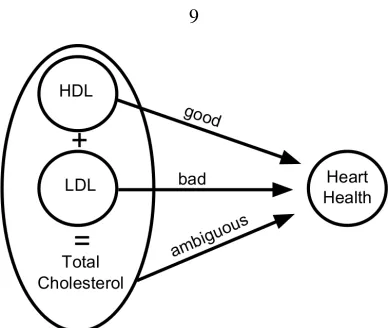
Figure 1.2: Ambiguous Manipulation. Total cholesterol is the sum of LDL and HDL. Suppose that LDL causes heart disease and HDL prevents it. The effect of total cholesterol on heart disease is then ambiguous as it depends on the proportion of HDL vs. LDL (see Sec.1.2.1). Experimental procedures based on adjusting total cholesterol only can give inconsistent results.
Consequently, to recommend a “low-cholesterol diet” is to prescribe anambiguous manipulation: “low-cholesterol” could mean low in LDL, HDL or both, but each would have very different consequences for the heart. Unless the proportions of LDL vs. HDL are known in advance, this makes a proper experimental verification of the causal link between total cholesterol and heart disease impossible. The example illustrates that there exists an appropriate “ground-truth” level of aggregation to describe the causal relation, and “total cholesterol” is too high-level. The challenge is to identify when one has reached the correct level.
CFL addresses this concern, and requires causal variables to be unambiguous: Each macrovariable state must have a consistent, well-defined causal effect. This effect can be probabilistic and highly variable, but must not depend on the microvariable instantiation of the macrovariable. For just like the specifics of gas molecule momenta do not change the effects of temperature, as long as their mean is equal. In this way, CFL abstracts microscopic details of the problem away, allowing the scientist to focus on all the relevant macroscopic details. This is analogous to the role of the macrovariables in Fig. 1.1 (A–C).
1.2.2
Macrovariables Are Task-Specific
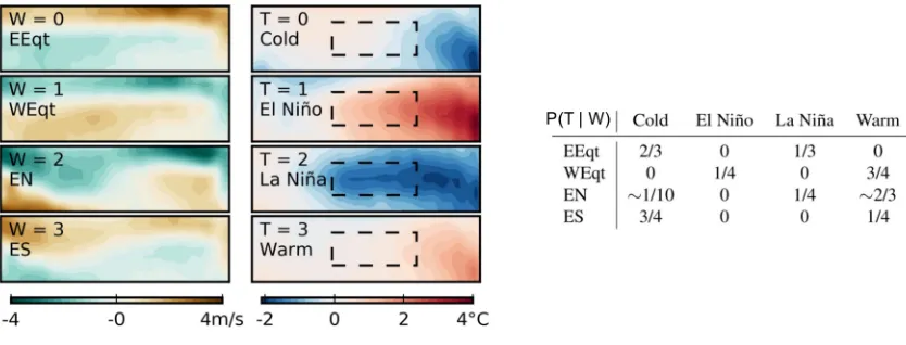
Figure 1.3: Macrovariables of Pacific Weather Patterns. A preview of the results of applying CFL to climate data in Chapter 5. The microvariables consist of zonal (East-West) wind strength over the equatorial Pacific and SST maps over the same region. The figure shows the causal hypothesis discovered by CFL. Each image represents one macrovariable state, the average over one cluster of windW (left) or temperature T (right). The conditional probability table showsP(T | W), the probability of the hypothesized SST macrovariable given the hypothesized wind macrovariable. It shows that CFL learned at least two relations that, causally interpreted, are consistent with current climate science: ‘Westerly winds’ (W=1) cause El Ni˜no (T=1) and ‘Easterly winds’ (W=0) cause La Ni˜na (T=2).
optic array, and the desired behavior), rather than by one or the other of the spaces considered individually. As an example, take ‘wind strength map over the Pacific Ocean’ as the input space, and ‘SST’ as the output space. Applying CFL to this task yields a discrete division of each space into a set of wind pattern classes (‘Westerly Winds’, ‘Easterly Winds’ etc) and SST pattern classes (‘El Ni˜no’, ‘La Ni˜na’ etc) – Chapter 5 describes the experiment in detail. Knowing which class a wind pattern belongs to then gives all the useful information about itspossibleeffects on SST1. For a different output space – say “average US income” – the input macrovariable would change, unless the causal consequences are entirely mediated by the same wind patterns.
1.3
Example Microvariable Cause-Effect Systems
The current section describes four example CFL problems. Further chapters develop the theory and algo-rithms necessary to solve these problems, and present experimental results. This section has two goals:
1. Clarify, by example, when CFL is useful, and 2. provide a guide to the contents of this book.
By necessity, most of our experiments are done on simulated systems. The reason is that the “causal ground-truth” can only be obtained either by definition of the system, or through thorough experimentation.
The latter is an expensive and time-consuming in most interesting cases. Nevertheless, Chapter 5 contains a limited application of the framework to real data where the ground-truth is given by expert opinion.
1.3.1
Images and a Spiking Neuron
Fig. 1.4 presents a cartoon of a paradigmatic case study in visual CFL. The contents of an imageIare caused by external, non-visual binary hidden variablesH1andH2such that ifH1 is on,I contains a vertical bar
(v-bar2) at a random position, and ifH
2 is on,Icontains a horizontal bar (h-bar) at a random position. A
target behaviorT ∈ {0,1}is caused byH1andI, such thatT = 1is more likely wheneverH1 = 1and
whenever the image contains an h-bar. T could indicate, for example, whether a particular neuron in the human brain significantly exceeds its baseline spiking rate within 500ms after viewing the image.
This example is deliberately constructed such that the visual cause is clearly identifiable: manipulating the presence of an h-bar in the image will influence the distribution ofT. Thus, we can call the following functionC:I → {0,1}thecausal featureofIor themacrovariable causeofT:
C(I) =
1 ifIcontains an h-bar
0 otherwise.
The presence of a v-bar, on the other hand, is not a causal feature. Manipulating the presence of a v-bar in the image has no effect onH1orT. Still, the presence of a v-bar is as strongly correlated with the value of
T (via the common causeH1) as the presence of an h-bar is. Call the following functionS:I → {0,1}the spurious correlateofT inI:
S(I) =
1 ifIcontains a v-bar
0 otherwise.
Both the presence of h-bars and the presence of v-bars are good individual (and even better joint) predic-tors of the target variable, but only one of them is a cause. Identifying the visual cause from the image thus requires the ability to distinguish among the correlates of the target variables those that are actually causal, even if the non-causal correlates are (possibly more strongly) correlated with the target.
Chapter 2 defines rigorously what it means to be a macrovariable cause and spurious correlate in a general setting. It provides theory and algorithms for optimal experimental design to differentiate the two. Chapter 4 describes a method to learn a manipulator function. The manipulator takes a microvariable input (for ex-ample, an image with a horizontal and vertical bar in it, as well as other, causally irrelevant, structure) and constructs theclosest possible(according to some metric) image that has a different causal effect. In our example, a perfect manipulator would remove only one pixel from the (causally relevant) h-bar to remove this feature of the image, but would leave any v-bars intact (since they are not causal features). As discussed in Chapter 4, manipulator functions make CFL useful in contexts where the goal is not only to understand
H1
H2 I T
P(H2=0) = 0.5
P(H1=0) = 0.5
P( I | H1=0, H2=0) = U( )
P( I | H1=0, H2=1) = U( )
P( I | H1=1, H2=0) = U( )
P( I | H1=1, H2=1) = U( )
P(T=0 | I ( , ), H1=0) = .33
P(T=0 | I ( , ), H1=1) = .66
P(T=0 | I ( , , ), H1=1) = 0
[image:17.612.213.437.224.427.2]P(T=0 | I ( , ), H1=0) = 1
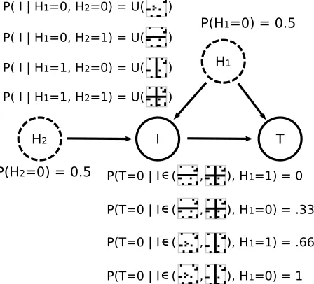
Figure 1.4:A Toy Causal Model of Visual Features Activating a Single Neuron.Two binary hidden (non-visual) variablesH1andH2toss unbiased coins. These variables represent random events in the world, e.g.
H1could mean “There is a tree nearby”. The content of the imageIdepends on these variables as follows.
IfH1=H2 = 0,Iis chosen uniformly at random from all the images containing no v-bars and no h-bars.
IfH1 = 0andH2 = 1,Iis chosen uniformly at random from all images containing at least one h-bar but
no v-bars. IfH1 = 1andH2= 0,Iis chosen uniformly at random from all the images containing at least
one v-bar but no h-bars. Finally, ifH1=H2= 1,Iis chosen from images containing at least one v-bar and
at least one h-bar. The distribution of the binary behaviorT depends only on the presence of an h-bar inI and the value ofH1. In observational studies,H1= 1iffIcontains a v-bar. However, amanipulationof any
specific imageI=ithat introduces a v-bar (without changingH1) will in general not change the probability
causal mechanisms of a system, but also manipulate the system efficiently. For example in healthcare, the desire to understand the relationship between the human body and its environment is driven by the underlying goal ofinterveningon the environment in order to improve health.
1.3.2
Hue and Skin Conductance
In the previous example, input images consisted of microvariables, but the output was a binary macrovariable. Sec. 1.2, however, motivated this work with many examples in which both the cause and the effect supervene on microvariables. In such cases it is not possible to “anchor” the discovery of causal features in a well-defined effect – both the cause and the effect have to be learned jointly. I call this the unsupervised CFL setting, in contrast to the supervised CFL described above.
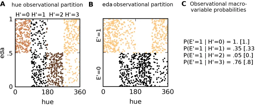
A simple toy example will visualize the definitions and main algorithmic steps involved in unsupervised CFL (we return to this example in Chapter 3). Take a fictitious study on the influence of color on the elec-trodermal activity (eda) (also known as the skin conductance). In a fictitious experiment, the elecelec-trodermal response to a (constant but unspecified) stimulus is recorded in varying environments. At the same time, the predominant hue of the environment is recorded. Our simulated system is pictured in Fig. 1.5. In the sys-tem, “Red” hues increase eda (a perhaps controversial but plausible response, see e.g. Jacobs and Hustmyer (1974)). In addition, living in warmer climates increases eda, but also increases the chance of observing “Warm” colors in the environment. Our imaginary study consists of picking humans from diverse popula-tions at random, and measuring their eda as well as the predominant hue in their environment. The example is set up to exhibit three characteristics:
1. The microvariables (hue and eda) are one-dimensional. Although this makes the example rather con-trived, the visualizations of the algorithms and definitions are much simpler and more illuminating than in higher-dimensional cases.
2. Microvariable hue gives rise to intuitive macrovariables: color classes. “Red” colors, “Natural” colors or “Warm” colors are (subjective) partitions of the hue space, and clearly superveneon hue. For example, “Red” is notcausedby hue, it is simply a range in the hue space.
3. The cause (hue) influences the effect (eda) by direct causation, but they are at the same time con-founded by geographic location. The goal of CFL is to separate the causal information and the purely-confounded information, and compress each into a separate macrovariable.
p(hue, eda) =X
lat
p(eda|hue, lat)p(eda|lat)p(lat). (1.1)
The probability tables for these factors are shown in Fig. 1.5. We purposefully constructed the conditional distributionp(eda|hue, lat)to take a special form: there are four ranges ofhuewithin whichp(eda|hue)
is constant. For example, the conditional is the same for anyhue∈(0,90). This construction indicates that there aremacrovariablesdriving the relation betweenhueandeda: to a good approximation, any hue within a given range has the same effect on eda. The situation is analogous to that of the temperature macrovariable driving the relation between, say, water and human pain receptors. The probability and intensity of experi-encing pain is roughly the same upon touching any body of water with the same temperature – given that all the other relevant variables, such as the individual experiencing pain, remain unchanged.
Chapter 3 shows that in unsupervised CFL tasks such as the one described in this section, causal macrovari-ables are unique and can be extracted automatically from the data. For now, we propose a “ground truth” macrovariable model that agrees with the microvariable distribution shown in Fig. 1.5. Chapter 3 shows that this model is in factthemacrovariable structure that supervenes onhueandedaand can be automatically discovered using CFL.
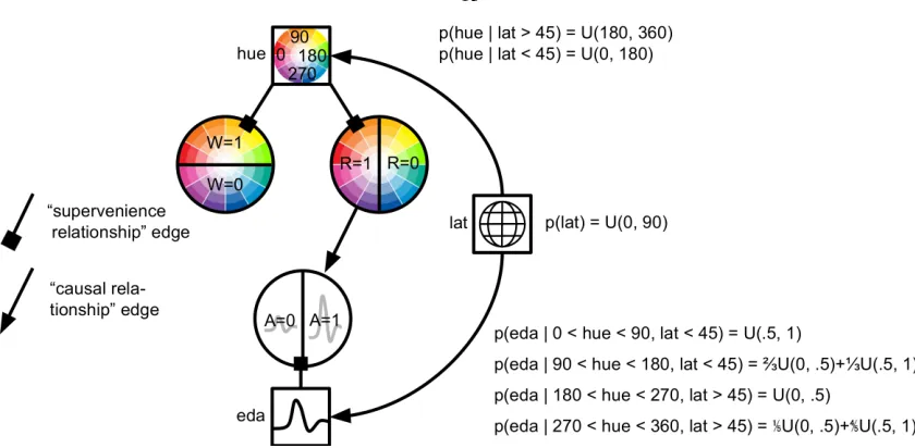
The macrovariables are all binary.Asupervenes (is a function of)eda, withA= 1if and only ifeda > .5. That is,Arepresents an “Above-average” skin conductance.Ais caused byR(“Redness”) which supervenes onhue,R= 1 ⇐⇒ hue∈(0,90)∪(270,360). In addition,Acorrelates with, but is notcaused by,W – another variable that supervenes onhue,W = 1 ⇐⇒ hue∈(0,180).W represents “Warm” hues.
The causal graph of R, W andA, shown in Fig. 1.5, is determined by the variables’ supervenience on hueandeda. Similarly, the joint probability distribution P(R, W, A)is fully determined byp(hue, eda). Algorithm 3 shows how to recover the variablesR andA– the causally relevant variables – through data-driven experimental design.
1.3.3
Images and Neural Populations
Whereas the above simulated dataset is simple and low-dimensional, unsupervised CFL can be applied to very high-dimensional and complex data. The current example is partially inspired by a problem at the core of much of modern neuroscience that is a generalization of the problem presented in Sec. 1.3.1: Can we detect which features of a visual stimulus result in particular responses ofneural populationswithout pre-defining the stimulus features or the types of population response we are interested in?
Figure 1.5: Causal Graphical Model of Color Influencing eda. In the simulated study, the predominant hue of the environment causes changes in the electrodermal response: red hues increase eda beyond the average, whereas non-red hues tend to decrease it. In addition, the latitude of the experiment influences eda: lower latitudes, close to the equator, cause higher absolute eda due to predominantly warm climate. Lower latitude visual environments tend also to have visually warmer hues, whereas higher latitude environments often have cooler hues. The probability tables show generative probabilities for our data, whereU(a, b)is the uniform distribution betweenaandb. For example, iflat >45and270 < hue <360, thenp(eda) =
.2U(0, .5) +.8U(.5,1)– a mixture of two uniform distributions that indicates that most likely, eda is above the average in this situation.
experimental protocol in the field: prepare stimuli that represent various hypotheses about what the neurons respond to; record from single or multiple units; and analyze the responses with respect to the candidate hypotheses.
But what if the candidate hypotheses are wrong? Or if they do not line up cleanly with the actually relevant features? CFL offers a less biased and more automatized process of experimentation: Record neural population responses to a broad set of stimuli. Then, jointly analyze what features of the stimuli modify responses of the neural populationandwhat features of neural activity are changing in response to the stimuli. To our knowledge, such joint cause-and-effect learning is a novel contribution not only in the neuroscientific setting, but to a whole array of other scientific disciplines.
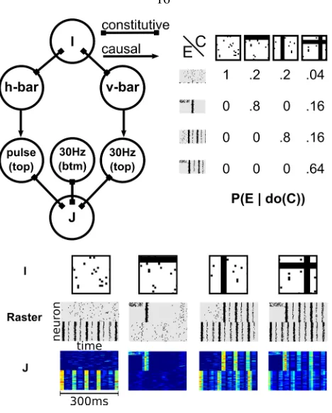
Figure 1.6: A simulated neuroscience experiment. A stimulus imageIcan contain a horizontal bar (h-bar), a vertical bar (v-bar), neither, or both (plus uniform pixel noise). In response to an image, a simulated population of neurons (the “top” population) can produce a single pulse of joint activity, a 30 Hz rhythm, both, or neither, with probabilitiesP(pulse| h-bar) = 0.8andP(30Hz | v-bar) = 0.8. These two causal mechanisms compose to yield the full response probability table shown in top right. In addition, another (“bottom”) population of neurons can exhibit a rhythmic activity independent of the stimulus image. The system’s outputJ is a 10ms-window running average of the neural rasters, with the neuron indices shuffled (as a neuroscientist has no a-priori knowledge of how to order neurons). Here we show exampleJ’s sorted by neuron id; we use the shuffled version in our experiments.
bar (v-bar), the same population synchronizes in a 30Hz rhythm after roughly the same delay. The remaining (“bottom half”) population acts independently of the visual stimuli (perhaps the experimenter unwittingly planted some of the electrodes in a non-visual brain area). Half the time these “distractor neurons” follow their spontaneous noisy dynamics, and half the time they synchronize to produce a rhythmic activity. One can think of this activity as being caused by internal network dynamics, extra-visual stimuli or any other cause, as long as it is independent of the image presented by the experimenter.
problem.
1.4
Related Work
Our framework draws heavily on ideas developed in computational mechanics (Shalizi, 2001; Shalizi and Crutchfield, 2001; Shalizi and Moore, 2003) and connects them with the framework of causal graphical models (Spirtes et al., 2000; Pearl, 2000). After discussing these two frameworks, this section briefly indicates several other related areas of machine learning and information theory.
1.4.1
Computational Mechanics
Our approach derives its theoretical underpinnings from the theory of computational mechanics (Shalizi, 2001; Shalizi and Crutchfield, 2001). In particular, computational mechanics defines macrovariable states in terms of equivalence classes of conditional probabilities. Definition 5 from Cosma Shalizi’s PhD disser-tation (Shalizi, 2001) is in fact equivalent to our definition of the observational state (Definition 1 in this book).
However, in computational mechanics macrovariables stop at the level of conditional probabilities and are meant to ‘summarize’ the phenomena rather than to support causal reasoning. Our work supports an explicitly causal interpretation by incorporating the possibility of confounding and interventions. We take the distinction between interventional and observational distributions to be one of the key features of a causal analysis. Thus, our Def. 1 is just a first step, leading later to the development of the Causal Class and the Causal Coarsening Theorem that relates observation and intervention.
1.4.2
Causal Graphical Models
The framework of causal graphical models (Spirtes et al., 2000; Pearl, 2000) provides the grounds for our understanding of causality. In this framework,X causesY ifP(Y | do(X)) 6= P(Y), where do()is an operator representing a randomized experiment. That is, one variable causes another if and only if after intervening on the first we see a (probabilistic) change in the value of the latter – while all the other relevant factors are kept constant. This definition captures a wide range of intuitions about causality, for example:
1. Atmospheric pressurecausesthe position of the needle of a barometer. This is because changing the atmospheric pressure would have an effect on the needle. However, the needle’s position is not a cause of atmospheric pressure. Tampering with the barometer will never cause a change in air pressure. 2. Whether it rains or notcorrelates with3 the position of the barometer’s needle, but there is no direct
causal relation between the two. This is because they have acommon cause, the atmospheric pressure.
3Throughout this book we will often use the expression “x correlates with y” to mean that the two variables are probabilistically
3. Position of a barometer’s needle is neither a cause nor effect of a probabilistically unrelated variable such as the outcome of a coin toss.
The field of causal graphical models concerns itself mainly with two tasks: 1) discovering the causal relation-ships between probabilistic variables (also called “learning the causal graph”), and 2) given a causal graph, inferring what effect a specific set of interventions will have on a chosen set of variables (classical approaches to these two problems are discussed broadly by Spirtes et al. (2000) and Pearl (2000)).
For our purposes, the above definition of causality is sufficient and we need not discuss causal discovery and inference further. We wish to remark, however, that the standard causal graphical models setting presup-poses that the relevant (macro)variables are given together with the problem specification. In contrast, in our setting the causal variables have to be constructed from the micro-variables they supervene on, before any causal relations can be established. This work is, as far as we know, the first attempt to construct meaningful causal variables from scratch, within the causal graphical models framework. We emphasize the difference between our method of causal featurelearningand methods for causal featureselection(Guyon et al., 2007; Pellet and Elisseeff, 2008). The latter choose the best (under some causal criterion) features from a restricted set of plausible macro-variable candidates. In contrast, our framework efficiently searches the whole space of all the possible macro-variables that can be constructed from an image.
1.4.3
Machine Learning and Artificial Intelligence
David MacKay ties together the fields of machine learning and information theory as follows (MacKay, 2003):
Why unify information theory and machine learning? Because they are two sides of the same coin. In the 1960s, a single field, cybernetics, was populated by information theorists, computer scientists, and neuroscientists, all studying common problems. Information theory and machine learning still belong together. Brains are the ultimate compression and communication systems. If machine learning is concerned with compression, the field of Artificial Intelligence (AI) is about how to use compression to act. Archetypical machine learning algorithms of the past two decades (neural net-works (Bishop, 1995), Support Vector Machines (Sch¨olkopf and Smola, 2001), Gaussian processes (Williams and Rasmussen, 2006)) can compress complex data all the way to the level of discrete labels or rid time-series of information irrelevant to a given predictive task. Thanks largely to the flexibility of neural net-works (Schmidhuber, 2015) and their commercialization however, we now see a revival of the desire to build agents endowed with the ability to act, at least in games (Silver et al., 2016; Mnih et al., 2013) – though the idea is certainly not new (Russell et al., 2003). Modern intelligent agents depend on machine learning when compressing information about their environment before acting.
interven-tions in the world, as well as the interveninterven-tions of other agents. We see our work as bridging causal inference and modern machine learning. Our work is all about how tocompressstimuli in order to get the most concise representation of thecausal mechanismsrelevant to a given task, and how toactorintervenein the world in an optimal manner, given that only low-level direct measurements are available. We use machine learning to create concise causal representations that can be directly used by intelligent agents to act in the world.
Chapter 2
Supervised Causal Feature Learning
This chapter develops the theory of supervised CFL within the context ofvisualcauses. This setting makes the definitions most intuitive and is itself of significant practical interest. A visual cause is defined (more formally below) as a function (orfeature) of raw image pixels that has acausal effecton a well-defined target behavior of a perceiving system of interest. However, the framework and results can be equally well applied to extract causal information from any aggregate of micro-variables on which manipulations are possible. Examples include auditory, olfactory and other sensory stimuli; high-dimensional neural recordings; market data in finance; consumer data in marketing. There, causal feature learning is both of theoretical (“What is the cause?”) and practical (“Can we automatically manipulate it?”) importance.
Visual perception is an important trigger of human and animal behavior. The visual cause of a behavior can be easy to define, say, when a traffic light turns green, or quite subtle: apparently it is the increased symmetry of features that leads people to judge faces more attractive than others (Grammer and Thornhill, 1994). Significant scientific and economic effort is focused on visual causes in advertising, entertainment, communication, design, medicine, robotics and the study of human and animal cognition. Visual causes profoundly influence our daily activity, yet our understanding of what constitutes a visual cause lacks a theoretical basis. In practice, it is well-known that images are composed of millions of variables (the pixels) but it is functions of the pixels (often called ‘features’) that have meaning, rather than the pixels themselves.
2.1
Advances in This Chapter
This chapter presents the following advances in machine learning and causal inference:
• The Causal Coarsening Theorem (CCT), which shows how observational data can be used to learn the visual cause with minimal experimental effort. CCT provides a connection between state-of-the-art machine learning methods for classification and causal discovery and experimental design.
• Algorithms to learn the visual cause from data and with minimal resort to experimentation.
2.2
Theory
Consider again the example from Sec. 1.3.1. There, the visual cause is identified with the presence of an h-bar. But the example does not provide a theoretical account of what it takes to be a visual cause in the general case when we do not know what the causally relevant pixel configurations are. In this section, we provide a general account of how the visual cause is related to pixel data.
2.2.1
Visual Causes as Macro-variables
A visual cause is a high-level random variable that is a function (or feature) of the image, which in turn is defined by the random micro-variables that determine the pixel values. The functional relation between the image and the visual cause is, in general, surjective, though in principle it could be bijective. While we are interested in identifying the visual causes of a target behavior, the functional relation between the image pixels and the visual cause should not itself be interpreted as causal. Pixels do notcausethe features of an image, theyconstitutethem, just as the atoms of a table constitute the table (and its features). The difference between the causal and the constitutive relation is that the former requires the possibility of independent manipulation (at least to some extent), whereas by definition one cannot manipulate the visual cause without manipulating the image pixels.
The probability distribution over the visual cause is induced by the probability distribution over the pixels in the image and the functional mapping from the image to the visual cause. But since a visual cause stands in a constitutive relation with the image, we cannot without further explanation describe interventions on the visual cause in terms of the standarddo-operation (Pearl, 2000). Our goal will be to define a macro-variable C, which contains all the causal information available in an image about a given behaviorT, and define its manipulation.
H1 H2
I T
HN
H = (H1, ... , HN)
[image:27.612.220.428.56.188.2]HC = (H2, HN)
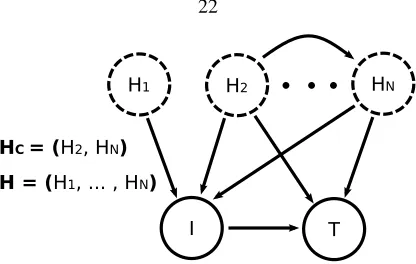
Figure 2.1: A general model of visual causation. In our model each imageIis caused by a number of hidden non-visual variablesHi, which need not be independent. The image itself is the only observed cause of a
target behaviorT. In addition, a (not necessarily proper) subset of the hidden variablesHCcan be a cause of
the target behavior. These confounders create visual “spurious correlates” of the behavior inI.
2.2.2
From Micro- to Macro-variables
LetT ∈ {0,1}represent a target behavior.1LetIbe a discrete space of all the images that can influence the target behavior (in our experiments in Section 2.4,Iis the space ofn-dimensional black-and-white images). We use the following generative model to describe the relation between the images and the target behavior: An image is generated by a finite set of unobserved discrete variablesH1, . . . , Hm(we writeHfor short).
The target behavior is then determined by the image and possibly a subset of variablesHc ⊆ Hthat are
confounders of the image and the target behavior:
P(T, I) =X
H
P(T |I,H)P(I|H)P(H)
=X
H
P(T |I,Hc)P(I|H)P(H). (2.1)
Independent noise that may contribute to the target behavior is marginalized and omitted for the sake of simplicity in the above equation. The noise term incorporates any hidden variables which influence the behavior but stand in no causal relation to the image. Such variables are not directly relevant to the problem. Fig. 2.1 shows this generative model.
Under this model, we can define anobservational partitionof the space of imagesIthat groups images into classes that have the same conditional probabilityP(T |I):
Definition 1(Observational Partition, Observational Class). Theobservational partitionΠo(T,I)of the set of imagesIw.r.t. behaviorT is the partition induced by the equivalence relation∼such thati∼j if and only ifP(T | I = i) = P(T | I = j).We will denote it asΠowhen the context is clear. A cell of an observational partition is called anobservational class.
In standard classification tasks in machine learning, the observational partition is associated with class
1An extension of the framework to non-binary, discreteT is easy but complicates the notation significantly. An extension to the
labels. In our case, two images that belong to the same cell of the observational partition assign equal
predictiveprobability to the target behavior. Thus, knowing the observational class of an image allows us to predict the value of T. However, the predictive probability assigned to an image does not tell us the
causaleffect of the image onT. For example, a barometer is widely taken to be an excellent predictor of the weather. But changing the barometer needle does not cause an improvement of the weather. It is not a (visual or otherwise) cause of the weather. In contrast, seeing a particular barometer reading may well be avisual causeof whether we pack an umbrella.
Our notion of a visual cause depends on the ability to manipulate the image.
Definition 2(Visual Manipulation). Avisual manipulationis the operation man(I = i)that changes (the pixels of) the image to imagei∈ I, while not affecting any other variables (such asHorT). That is, the manipulated probability distribution of the generative model in Eq.(2.1)is given byP(T | man(I =i)) =
P
HcP(T |I=i,Hc)P(Hc)(see Pearl (2000) for a detailed discussion of the probabilistic interpretation
of causal manipulation).
The manipulation changes the values of the image pixels, but does not change the underlying “world”, represented in our model by theHi that generated the image. Formally, the manipulation is similar to the
do-operator for standard causal models. However, in this book we reserve thedo-operation for interventions on causalmacro-variables, such as the visual cause ofT. We discuss the distinction in more detail below.
We can now define thecausal partitionof the image space (with respect to the target behaviorT) as: Definition 3(Causal Partition, Causal Class). The causal partitionΠc(T,I)of the setIw.r.t. behaviorT is the partition induced by the equivalence relation∼defined onIsuch thati∼jif and only ifP(T |man(I=
i)) = P(T |man(I = j))fori, j ∈ I. When the image space and the target behavior are clear from the context, we will indicate the causal partition byΠc. A cell of a causal partition is called acausal class.
The underlying idea is that images are considered causally equivalent with respect toT if they have the same causal effect onT. Given a causal partition of the image space, we can now define the visual cause of T:
Definition 4(Visual Cause). Thevisual causeC of a target behaviorT is a random variable whose value stands in a bijective relation to the causal class ofI.
2.2.3
The Causal Coarsening Theorem
The main theorem of this book relates the causal and observational partitions for a givenI andT. It turns out that under appropriate, intuitive assumptions, the causal partition is a coarsening of the observational partition. That is, the causal partition aligns with the observational partition, but the observational partition may subdivide some of the causal classes.
2.2.4
Set-up and Definitions
For simplicity, consider a causal system between three discrete variablesH, I, T in whichIandH are both causes ofT, andHis in addition a cause ofI– equivalent to the setup in Fig. 2.1 but with all the confounders collapsed into one variable for simplicity of notation. We assume that these three variables fully describe the causal system, that is, with respect to these three variables the system is causally sufficient. (In fact, since we treatH as an unobserved common cause ofIandT,Hcan be thought of as a catch-all for any confounding betweenIandT.) The parameterization of this causal system is given by
P(H, I, T) =P(H)P(I|H)P(T |I, H). (2.2)
We define partitions of the micro-variable spaceI.
Definition 5(partitionΠf(I)). LetΠf(I)to be the partition onI induced by the relationshipi1 ∼ i2 ⇔
f(i1) =f(i2)for anyi1, i2∈ I.
Here f stands for any function whose domain contains I. For exampleP(H | I)or P(I)are such functions, where i1 ∼ i2 means thatP(H | i1) = P(H | i2)for any value ofH. Thus the causal and
observational partition above can be rewritten as, respectively
Πc(I) = ΠP(T|man(I))(I) (2.3)
Πo(I) = ΠP(T|I)(I) (2.4)
We writeC(i)to denote the causal class ofi inΠc(I)andO(i)to denote the observational class ofiin
Πo(I).
In addition, we will make use below of a partition ΠP(I|H)(I), that we refer to as the confounding
partition:
i1∼i2 ⇔ P(i1|H) =P(i2|H) ∀h∈H.
P(T=0 | do{ }) = .17
P(T=0 | do{ }) = .83
P(T=0 | ) = .33
P(T=0 | ) = .66 P(T=0 | ) = 0
P(T=0 | ) = 1
Figure 2.2: The Causal Coarsening Theorem. The observational probabilities of T givenI (gray frame) induce an observational partition on the space of all the images (left, observational partition in gray). The causal probabilities (red frame) induce a causal partition, indicated on the left in red. The CCT allows us to expect that the causal partition is a coarsening of the observational partition. The observational and causal probabilities correspond to the generative model shown in Fig. 1.4.
Theorem 6(Causal Coarsening Theorem). Among all the joint distributionsP(T, H, I)over discrete vari-ablesT, H, I, consider the subset that induces any fixed causal partitionΠc(I)and a fixed confounding partitionΠP(T|I)(I). Within this subset, the set of distributions whose causal partitionΠc(I)is not a coars-ening of the observational partitionΠo(I)is a set of measure zero.
Fig. 2.2 illustrates the relation between the causal and the observational partition implied by the theorem. We prove the CCT in Sec. 2.5.
The motivation for the CCT is to establish a connection between the observational partitionΠo(I)and
the causal partitionΠc(I)such that minimal experimental effort is required to learn the causal partition
given an observational partition. In particular, if the observational partition already constitutes a coarsening of the micro-variable spaceI, then the hope was to leverage this coarse observational partition to learn the causal partition. Consequently, in order to obtain any experimental savings from the developed algorithms we require a theorem that establishes a connection between an observational partition that is itself already a coarsening of the micro-variable spaceI, and the the causal partition.
An observational partition that is a coarsening of the micro-variable spaceIcan arise for several reasons, To have such a coarsening, the following equation must be satisfied for at least two distincti1, i2∈ I:
P(T |i1) =P(T |i2) (2.5)
⇔X
H
P(T |i1, H)P(H |i1)−P(T |i2, H)P(H |i2) = 0
⇔X
H
P(H)(P(T |i1, H)P(i1|H)−P(T |i2, H)P(i2|H)) = 0
⇔X
H
P(T |i1, H)P(i1|H)−P(T |i2, H)P(i2|H) = 0 (2.6)
SinceHis assumed to be a hidden variable there is no significance to states that have zero probability, so the assumption on the last line is innocuous. Note that equation 2.6 is stated entirely in terms of the fundamental parameters in equation 2.2.
Consequently, for an observational partition to be a coarsening of the micro-variable space, the fundamen-tal parameters must combine in just such a way that equation 2.6 is satisfied. However, there is an important subclass of such combinations that satisfy the equation due to the fact that the corresponding fundamental parameters fori1andi2are equal, i.e. when
P(T |i1, H) =P(T |i2, H) ∀h∈H
P(i1|H) =P(i2|H) ∀h∈H
It is these cases that are of interest to the discovery of causal macro-variables, since – intuitively – the coarseness of the observational partition arises from causal effects that are invariant across distinctions at the micro-level – this is the case in all the simulated examples enumerated in Chapter 1. In other cases that satisfy equation 2.6, the parameters just happen to combine in such a way as to result in a coarse observational partition.
The CCT shows that no matter what partitions we fixΠcandΠP(I|H)to, the set of distributions
consis-tent with these partitions has the property that the causal partition will be a coarsening of the observational partition except for a set of distributions that has measure zero.
In particular, if we assume that the observational partition is a coarsening ofI only becauseboth the confounding partition ΠP(I|H) and the causal partition ΠP(T|man(I)) are each coarsenings of I, then the
theorem justifies the application of the algorithms developed in the following section to problems where the observational partition is itself already a coarsening of the micro-variable space ofI. In other words, when using CFL we assume away cases where a coarse observational partition arises due to “coincidental” combinations of the fundamental parameters that satisfy Equation 2.6. Finally, the notion of coincidence here is not measure-theoretic in the standard sense, since for two fundamental parameters to be equal carries in a standard measure-theoretic analysis the same amount of measure as the event that a combination of parameters satisfy a particular algebraic constraint. However, our set-up takes as starting point the assumption that there exist causal macro-variables in nature. In that case, the equality of two fundamental parameters P(T |h, i1) =P(T |h, i2)is not coincidental but a result of a macro-variable, whereas the satisfaction of
2.2.5
The Complete Macro-variable Description Theorem
Recall the example from Sec. 1.3.1, where the visual presence of an h-bar causes a neuron to spike, and the presence of a v-bar correlates with the spiking only through a confounder. In this section, we formalize the intuition that the v-bar is a visualspurious correlateof neural spiking.
Assume that the causal partitionΠT
c is a coarsening of the observational partitionΠTo, in accordance
with the CCT. Each of the causal classes c1,· · ·, cK delineates a region in the image space I such that
all the images belonging to that region induce the sameP(T | man(I)). Each of those regions—say, the k-th one—can be further partitioned into sub-regionssk1,· · ·, skM
k such that all the images in the m-th sub-region of the k-th causal sub-region induce the same observational probabilityP(T | I). By assumption, the observational partition has a finite number of classes, and we can arbitrarily order the observational classes within each causal class. Once such an ordering is fixed, we can assign an integerm∈ {1,2,· · ·, Mk}to
each imageibelonging to the k-th causal class such thatibelongs to the m-th observational class among theMk observational classes contained inck. By construction, this integer explains all the variation of the
observational class within a given causal class. This suggests the following definition:
Definition 7(Spurious Correlate). Thespurious correlateS is a discrete random variable whose value dif-ferentiates between the observational classes contained in any causal class.
The spurious correlate is a well-defined function on I, whose value ranges between1 andmaxkMk.
LikeC, the spurious correlateSis a macro-variable constructed from the pixels that make up the image.C andStogether contain all and only the visual information inIrelevant toT, but onlyCcontains the causal information:
Theorem 8 (Complete Macro-variable Description). The following two statements hold forC and S as defined above:
1. P(T |I) =P(T |C, S).
2. Any other variableXsuch thatP(T |I) =P(T |X)has entropyH(X)≥H(C, S).
We prove the theorem in Sec. 2.5. It guarantees that C andS constitute the smallest-entropy macro-variables that encompass all the information about the relationship betweenT andI. Fig. 2.3 shows the relationship between C, SandT, the image spaceI and the observational and causal partitions schemat-ically. C is now a cause of T, S correlates withT due to the unobserved common causesHC, and any
information irrelevant toT is pushed into the independent noise variables (commonly not shown in graphical representations of structural equation models).
Figure 2.3: A macro-variable model of visual causation. Using our theory of visual causation we can ag-gregate the information present in visual micro-variables (image pixels) into the visual causeCand spurious correlateS. According to Theorem 8,CandScontain all the information aboutT available inI.
causes, but it does not (directly) affect the other variables in the system or the relationships between them (see themodularity assumptionin Pearl (2000)). However, unlike the standard case where causal variables are separated in location (e.g.smokingandlung cancer), the causal variables in an image may involve the same pixels:Cmay be the average brightness of the image, whereasSmay indicate the presence or absence of particular shapes in the image. An intervention on a causal variable using thedo-operator thus requires that the underlying manipulation of the image respects the state of the other causal variables:
Definition 9(Causal Intervention on Macro-variables). Given the set of macro-variables{C, S}that take on values{c, s}for an imagei ∈ I, an intervention do(C =c0)on the macro-variableCis given by the manipulation of the image man(I =i0)such thatC(i0) =c0andS(i0) =s. The intervention do(S =s0)is defined analogously as the change of the underlying image that keeps the value ofCconstant.
In some cases it can be impossible to manipulate C to a desired value without changing S. We do not take this to be a problem special to our case. In fact, in the standard macro-variable setting of causal analysis we would expect interventions to be much more restricted by physical constraints than we are with our interventions in the image space. This issue is ultimately quite subtle both from the philosophical and practical point of view. We do not discuss it in full detail here, as the details of the discussion may vary significantly between various domains.
2.2.6
Predictive Non-causal Information in the Macro-variable Cause
In some casesCretains predictive information that is not causal. Consider the following example: We have a causal graph consisting of three variables{I, T, H}where the causal relations areI→T andI←H →T. All three variables are binary and we have a positive distribution over the variables. In the general case, distributions over this graph satisfy
2. P(T|I= 1)6=P(T|I= 0), and importantly 3. P(T|I)6=P(T|do(I)).
If we viewI as an image (which can either be all black or all white),T as the target behavior andH as a hidden confounder, analogous to the set-up in the main article, then the observational partitionΠohas just
two classes, namely{1,0}. But in this case the observational partitionis the sameas the causal partition:
Πo= Πc. So by our definition of a spurious correlate,Sis a constant, since there are no further distinctions to
be made within any of the causal classes.Swould be omitted from any standard causal model. Nevertheless, we have in our model still thatP(T|C) 6=P(T|do(C)), i.e. the causal variableCstill contains predictive information that is not causal. Given that there is by construction no other than the causal and the trivial partition in this example, it must be the case thatCretains predictive non-causal information. It follows that in our definitions ofC andS, it is not the case that the predictive non-causal components of an image can always be completely separated from the causal features. However, any distinction we make inCdoes make a causal difference.
2.3
Algorithms
The theoretical advances of the previous section allows us to develop algorithms to learnC, the visual cause of a behavior. In addition, knowledge ofCwill allow us to specify amanipulator functionwhich we discuss separately in Chapter 4.
2.3.1
Predicting Macro-variable Intervention Results
A standard machine learning approach to learning the relation betweenI andT would be to take an ob-servational datasetDobs ={(ik, P(T | ik))}k=1,···,N and learn a predictorf whose training performance
guarantees a low test error (so thatf(i∗)≈P(T |i∗)for a test imagei∗). In causal feature learning, low test error on observational data is insufficient; it is entirely possible thatDcontains spurious information useful in predicting test labels which is nevertheless not causal. That is, the prediction may be highly accurate for observational data, but completely inaccurate for a prediction of the effect of a manipulation of the image (recall the barometer example). However, we can use the CCT to obtain a causal dataset from the observa-tional data, and then train a predictor on that dataset. Algorithm 1 uses this strategy to learn a functionC that, presented with any imagei ∈ I, returnsC(i)≈P(T | man(I =i)). We use a fixed neural network architecture to learnC, but any differentiable hypothesis class could be substituted instead. Differentiability ofCis necessary in Section 4.3 in order to learn the manipulator function.
Algorithm 1:Causal Predictor Training
input :Dobs={(i1, p1=p(T |i1)),· · ·,(iN, pN =p(T |iN)}– observational data
P ={P1,· · ·, PM}– the set of observational classes (so that∀k, pk∈ P,1≤k≤N)
Train– a neural net training algorithm output:C: I →[0,1]– the causal variable
1 Pick{ik1,· · · , ikM} ⊂ {i1,· · · , iN}s.t.pkm =Pm; 2 EstimateCˆm←P(T |man(I=ikm))for eachm; 3 For allkletCˆ(ik)←Cˆmifpk=Pm;
4 Dcsl← {(i1,Cˆ(i1)),· · ·,(iN,Cˆ(iN))};
5 C←Train(Dcsl);
to know thatP(T | man(I =i)) = ˆCmfor any otheriin the same observational class. The choice of the
experimental method of estimating the causal class in Step 2 is left to the user and depends on the behaving agent and the behavior in question. If, for example,Trepresents whether the spiking rate of a recorded neuron is above a fixed threshold, estimatingP(T |man(I=i))could consist of recording the neuron’s response to iin a laboratory setting multiple times, and then calculating the probability of spiking from the finite sample. The causal dataset created in Step 4 consists of the observational inputs and their causal classes. The causal dataset is acquired throughO(N)experiments, whereN is the number of observational classes. The final step of the algorithm trains a neural network that predicts the causal labels on unseen images. The choice of the method of training is again left to the user.
2.4
Experiments
Section 4.4 contains experiments shared between this chapter and Chapter 4.
2.5
Proofs
Before proving the CCT, we prove a useful lemma.
Lemma 10. Let SP(H) denote the simplex of multinomial distributions over the values ofH. For fixed
P(T |H, I), the subset ofSP(H)for whichΠcis not equal toΠP(T|H,I)(I)is measure zero. Proof. We want to show that the subset ofSP(H)for which, for anyi1, i2∈ Iandh∈H
P(T |H=h, i1)6=P(T |H =h, i2), and (2.7)
P(T |man(i1)) =P(T |man(i2)), (2.8)
is measure zero. (Note that ifP(T |H, I)is the same for alli, equality ofΠcandΠP(T|H,I)follows directly
Eq. 2.8 is equivalent toP
hP(H=h)[P(T |H =h, i1)−P(T |H =h, i2)] = 0. Since this is a linear
constraint onSP(H), in order to show that it is satisfied on a measure-zero subset we only need to show that
there is at least one point which does not satisfy it.
First, set P(H = h) = 1/K, whereK is the number of states of H, for all h. If the equation is not satisfied, we are done. If it is satisfied, it must be for some h1 that P(T | H = h1, i1)−P(T |
H = h1, i2) > 0 and for some h2, we have P(T | H = h2, i1)−P(T | H = h2, i2) < 0. Pick
any 0 < < min(1/K,1−1/K). SetP(H = h1) = 1/K + andP(H = h2) = 1/K−, and
P(H =h) = 1/Kfor otherh. Then Eq. (2.8) does not hold.
Theorem (Causal Coarsening)Among all the joint distributionsP(T, H, I)over discrete variablesT, H, I, consider the subset that induces any fixed causal partitionΠc(I)and a fixed confounding partitionΠP(T|I)(I).
Within this subset, the set of distributions whose causal partitionΠc(I)is not a coarsening of the
observa-tional partitionΠo(I)is a set of measure zero.
Proof. (i) We first set up the notation. Assume thatT is binary, and thatHandIare discrete variables (say |H|=K,|I|=N, thoughNcan be very large).P(T |H, I)requiresK×Nparameters,P(I|H)requires
(N−1)×Kparameters, andP(H)requires anotherK−1parameters. Call the parameters, respectively,
αh,i,P(T = 0|H =h, I =i)
βi,h,P(I=i|H =h)
γh,P(H =h)
We will denote parameter vectors as
α= (αh1,i1,· · ·, αhK,iN)∈R
K×N
β = (βi1,h1,· · ·, βiN−1,hK)∈R
(N−1)×K
γ= (γh1,· · · , γhK)∈R
K−1,
where the indices are arranged in lexicographical order. This creates a one-to-one correspondence of each possible joint distributionP(T, H, I)with a point(α, β, γ)∈P[α, β, γ]⊂RK
2×(K−1)×N×(N−1)
.
(ii) Show that for any α, β consistent withΠc andΠP(I|H), the causal partition and the confounding
partition are, in general, fixed.
To proceed with the proof, pick any point in theP(T |H, I)×P(I|H)space – that is, fixαandβ. The only remaining free parameters are now inγ. Varying these values creates a subset of the space of all joints isometric to the(K−1)-dimensional simplex of multinomial distributions overKstates (call the simplex SK−1):
Note that fixingβdirectly fixesΠP(I|H). Fixingαdoesn’t directly fixΠc. But by Lemma 10, foralmost all
distributions inP[γ;α, β]the causal partitionΠc equals the partitionΠP(T|H,I), which is directly fixed by
α. LetP0[γ;α, β]beP[γ;α, β]minus this measure zero subset.
The statement of the theorem fixes Πc andΠP(I|H). If the α, β we picked are consistent with these
partitions withinP0[γ;α, β], continue with the proof. Otherwise, choose otherα, β.
We now prove that withinP0[γ;α, β]the set ofγfor which the causal partitionΠcis not a coarsening of
the observational partitionΠois of measure zero. Later in (iv) we integrate the result over allα, β.
(iii) Let the causal coarsening constraint be that fori1, i2∈ Iwe have
O(i1) =O(i2) ⇒ C(i1) =C(i2). (2.9)
That is, it is not the case that two members ofI are observationally equivalent but have causally different effects.
We show that the causal coarsening constraint holds for each pair i1, i2 ∈ I: Pick anyi1, i2 ∈ I. If
C(i1) = C(i2), then we are done with this pair. So assume that there is a causal difference, i.e.C(i1)6=
C(i2). Our goal is now to show that then only a measure-zero subset ofP0[γ;α, β]allows forO(i1) =O(i2).
We first show thatO(i1) =O(i2)places a polynomial constraint onP0[γ;α, β]. We have
O(i1) =
1
P(i1) X
h
αh,i1βi1,hγh,
O(i2) =
1
P(i2) X
h
αh,i2βi2,hγh.
After expanding in terms ofα, β, γ, we have
O(i1) =O(i2) ⇔ X
hk,hl
γhkγhl[βi2,hkβi1,hlαhl,i1−βi1,hkβi2,hlαhl,i2] = 0. (2.10)
We have thus shown that, for fixedα, βandi1, i2, the violation of the causal coarsening constraint (2.9),
is a polynomial constraint onP0[γ;α, β]. By an algebraic lemma (proven by Okamoto, 1973), the subset on which the constraint holds is measure zeroif the constraint is not trivial. That is, we only need to find oneγ for which Eq. (2.10) does not hold to prove that it almost never holds.
To find suchγ, letγh= 1/Kfor allh. If for thisγEq. (2.10) does not hold, we are done. If it does hold,
since we knowαis not all0, there must be in the sum of the equation at least one factor[βi2,hkβi1,hlαhl,i1−
βi1,hkβi2,hlαhl,i2]which is positive, and one that is negative. Call thehk, hlcorresponding to the positive
elementhk+, hl+and to the negative elementhk−, hl−. Since the factors are different, we must have either k+ 6=k− orl+ 6=l−(or both). Assumek+ 6=k−. Now, pick any positive < min(1/K,1−1/K). Set γh = 1/K for allh6=hk+, hk− and setγh
k+ =
1
K +andγhk− =
1
K −. In this way, we keep P
unchanged, and are guaranteed that Eq. (2.10) does not hold. That is, for thisγwe haveO(i1)6=O(i2)2.
(iv) Show that the theorem holds over the space of all distributions. To reiterate proof progress thus far:
1. We fixed the macro-scale causal partitionΠcand the confounding partitionΠP(I|H)and picked
arbi-traryαandβcompatible with these partitions. 2. We picked two pointsi1, i2for whichC(i1)6=C(i2).
3. We showed that for any such two points, the subset ofP0[γ;α, β]for whichO(i1) =O(i2)is measure
zero.
Since there are only finitely many points inI, it follows that for the fixedα, β, the subset ofP0[γ;α, β]on which the coarsening constraint (2.9 does not hold for at least one pair of points is also measure zero. Since P[γ;α, β]−P0[γ;α, β]is a set of measure zero, the subset ofP[γ;α, β]on which the causal coarsening constraint does not hold is also measure zero.
Now, call the set of all joint distributions that agree withΠc andΠP(I|H) the admissible set, and
de-note it withP[α, β, γ]A. For eachα, βconsistent with the two partitions, call the (measure zero) subset of
P[γ;α, β]Athat violates the causal coarsening constraintz[α, β]. LetZ =∪α,βz[α, β]⊂P[α, β, γ]Abe the
set of all the admissible joint distributions which violate the causal coarsening constraint. We want to prove thatµ(Z) = 0, whereµis the Lebesgue measure. To show this, we will use the indicator function
ˆ
z(α, β, γ) =
1 ifγ∈z[α, β],
0 otherwise.
By basic properties of positive measures we have
µ(Z) =
Z
P[α,β,γ]A
ˆ
z dµ.
For simplicity of notation, let
1. A ⊂RK×N be the set of all possibleα’s (a Cartesian product ofK×N 1-d simplexes);
2. B ⊂RN×Kbe the set of all possibleβ’s (a Cartesian product ofKsimplexes, eachN−1dimensional); 3. G ⊂RKbe the set of all possibleγ’s (aK−1-dimensional simplex).
Note that each set has, in its respective Euclidean space, a non-empty interior, and comes equipped with the Lebesgue measure.
Finally, letIA(α, β)be the indicator function that evaluates to1ifα, βare admissible and evaluates to0
otherwise. We have
Z
P[α,β,γ]A
ˆ
z dµ=
Z
A×B×G
ˆ
z(α, β, γ)IA(α, β)d(γ, β, α)
=
Z
A×B
Z
G
ˆ
z(α, β, γ)d(γ)IΠc(β, α)d(β, α)
=
Z
A×B
µ(z[α, β])IA(α, β)d(β, α) (2.11)
=
Z
A×B
0IA(α, β)d(β, α)
= 0.
Equation (2.11) follows aszˆrestricted toP[γ;α, β]is the indicator function ofz[α, β].
This completes the proof thatZ, the set of joint distributions overT, H andI that violate the causal coarsening constraint (2.9) is measure zero.
Theorem (Complete Macro-variable Description)The following two statements hold forCandSas de-fined in Sec. 2.2.5:
1. P(T |I) =P(T |C, S).
2. Any other variableXsuch thatP(T |I) =P(T |X)has Shannon entropyH(X)≥H(C, S). Proof. The first part follows by construction ofS. For the second part, note that by the CCT there is a bijective correspondence between the pairs of values(c, s)and the observational probabilities P(T | I). Call this correspondencef, that isf(c, s) = P(T | c, s)andf−1(p) ={c, s | P(T|c, s) =p}. Further,
definegas the function onX such thatg: x 7→ P(T | x). But sinceP(T | X) = P(T | I), we have
(c, s) =f−1(g(x)). That is, the value ofCandSis a function of the value ofX, and thus the entropy ofC
andSis smaller than or equal to the entropy ofX.
2.6
Additional Acknowledgement
Chapter 3
Unsupervised Causal Feature Learning
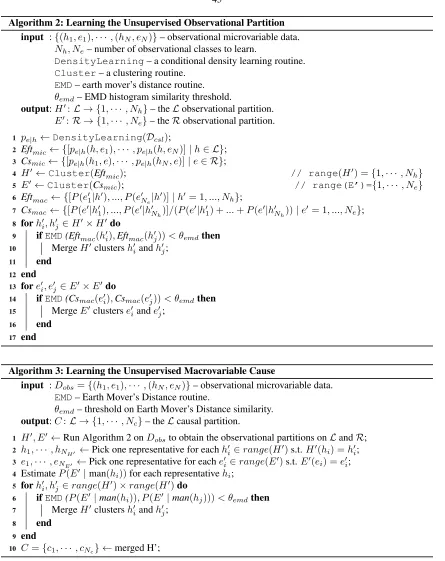
The previous chapter develops a method to discover from micro-variable data the macro-variable cause of a pre-defined macro-variable “target behavior”. In this chapter, we do not assume that the macro-level effect is already specified. Instead, in a generalization of the CFL framework, we simultaneously recover the macro-level cause C and macro-level effectE from micro-variable data. We will use the name Causal Feature Learning to refer to both frameworks. When ambiguous, we will refer to the first as supervised, and the current chapter’s as unsupervised CFL.
3.1
Advances in This Chapter
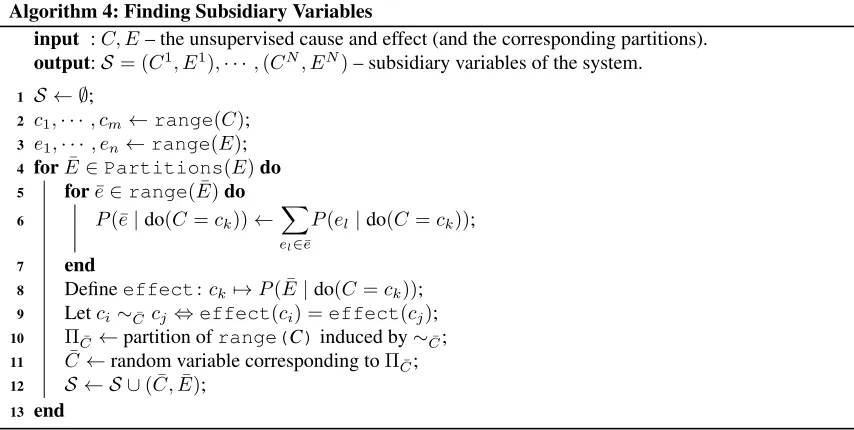
This chapter presents the following advances in machine learning and causal inference: