Globally Convergent Algorithms for DC Operating
Point Analysis of Nonlinear Circuits
Duncan A. Crutchley and Mark Zwolinski, Senior Member, IEEE
Abstract—An important objective in the analysis of an electronic
circuit is to find its quiescent or dc operating point. This is the starting point for performing other types of circuit analysis. The most common method for finding the dc operating point of a non-linear electronic circuit is the Newton–Raphson method (NR), a gradient search technique. There are known convergence issues with this method. NR is sensitive to starting conditions. Hence, it is not globally convergent and can diverge or oscillate between solutions. Furthermore, NR can only find one solution of a set of equations at a time. This paper discusses and evaluates a new ap-proach to dc operating-point analysis based on evolutionary com-puting. Evolutionary algorithms (EAs) are globally convergent and can find multiple solutions to a problem by using a parallel search. At the operating point(s) of a circuit, the equations describing the current at each node are consistent and the overall error has a min-imum value. Therefore, we can use an EA to search the solution space to find these minima. We discuss the development of an anal-ysis tool based on this approach. The principles of computer-aided circuit analysis are briefly discussed, together with the NR method and some of its variants. Various EAs are described. Several such algorithms have been implemented in a full circuit-analysis tool. The performance and accuracy of the EAs are compared with each other and with NR. EAs are shown to be robust and to have an ac-curacy comparable to that of NR. The performance is, at best, two orders of magnitude worse than NR, although it should be noted that time-consuming setting of initial conditions is avoided.
Index Terms—Circuit simulation, dc circuit analysis, differential
evolution, evolution strategies, tournament selection.
I. INTRODUCTION
T
HE FIRST task in simulating the behavior of a circuit is to find the quiescent or dc operating point. This is important because the operating point is required when performing other types of circuit analysis. For example, the dc operating point is used as the starting point for transient analysis (circuit response in the time domain) [1]. Circuit design algorithms also need the dc operating point of the circuit. In this case, the operating point is required to evaluate the dc performance of the current design under a given set of constraints on the circuit’s components [1]. Traditionally, the operating point is found by using the Newton–Raphson method (NR). This method has three po-tential problems. The first problem is that, at the start of each iteration, we must recompute the Jacobian matrix. The Jaco-bian matrix contains all the partial derivatives of the nonlinear device equations with respect to the circuit variables, nodeManuscript received August 27, 2001; revised January 29, 2002. This work was supported by the Engineering and Physical Sciences Research Council.
The authors are with the Department of Electronics and Computer Science, University of Southampton, Southampton SO17 1BJ, U.K.
Digital Object Identifier 10.1109/TEVC.2002.804319
voltages, and/or branch currents, which is computationally costly. The second problem is that the solution can diverge or fail to converge by oscillating between several potential solutions. This latter situation can occur in circuits with a large amount of feedback.
Finally, convergence is only guaranteed if a suitable initial so-lution vector is chosen. For circuits with more than one possible solution, the initial guess can influence the final solution and hence finding multiple global solutions is generally difficult. For example, an RS latch, which is a common subcircuit found in computer memory, has three potential solutions. NR-based al-gorithms will usually only find the metastable solution unless the user intervenes. This solution represents the latch in a bal-anced state, but it is often more important to know what the cir-cuit does in its two other conjugate state outputs at logic (1,0) in one case and (0,1) in the other. Obviously, these solutions would give three different starting points for a transient analysis. Hence, the ability to find multiple dc operating points, when they exist, can prove very useful for determining the behavior of the circuit over time.
In this paper, we discuss various aspects of evolutionary com-puting (EC), in particular evolution strategies (ESs), and differ-ential evolution (DE), and how these techniques can be applied to dc circuit analysis. As will be seen, EC has certain advantages over NR. The main benefits are improved convergence and the ability to find multiple solutions. These can be attributed to the parallel nature of EC algorithms, i.e., a search through a pop-ulation of solutions rather than a sequential search for an indi-vidual solution, as in NR. There are further adaptations that can be made to ES, such as more sophisticated mutations and se-lection schemes. At present, the alternatives to NR are slow, in part because of the way in which the algorithms have been im-plemented. We will also see that evolutionary algorithms (EAs) can find solutions to circuits that fail (without user intervention) when using NR.
At the end of this paper we will discuss of the results ob-tained from a SPICE-compatible evolutionary circuit simulator [evolutionary analog circuit simulator (EACS)] that implements versions of the basic EAs, including some more sophisticated features such as tournament selection and higher configurability with regard to the evolutionary operators and how they are used. Before continuing with a detailed look at the techniques outlined above, we will define the notation that is to be used throughout this work. In the NR algorithm, we represent the trial solutions, e.g., the vector of node voltages and/or branch currents, as a real-valued trial vector , at iteration . In general, the aim is to find a set of variables such that, for some objective function
, we have 0. In the case of EAs, the trial vector has an extra superscript that denotes the th member of the population. denotes the generation count and, thus, the trial
vector is written as . Without loss of
generality, we can restrict ourselves to the task of minimization because maximizing a function is the same as
mini-mizing , where in general and .
In the case of circuit analysis, the objective function is a vector representing the characteristic equations of the nonlinear circuit components. In EAs, the objective function represents the fitness of a particular trial vector.
It is important at this point to comment on the nature of the problem that is addressed in this paper. NR is used to find the roots of an equation or a set of equations, and as such this is not a minimization problem. We can, however, convert the root-finding problem of operating-point analysis into a minimiza-tion problem by specifying a fitness funcminimiza-tion and attempting to minimize that. This enables us to use EAs, which are search techniques that easily lend themselves to solving minimization problems.
II. CONVENTIONALCIRCUITANALYSISTECHNIQUES
In this section, we discuss the NR method for dc analysis. Conventionally, one analyzes a circuit to find its node voltages using Kirchhoff’s Current Law (KCL) [1]. A node voltage is calculated with respect to a common reference point. Sometimes a branch current is also required; in which case, Kirchhoff’s Voltage Law (KVL) is used [1]. A branch current is the current flowing between two nodes in the circuit. Before continuing, it is important to define KCL and KVL. KCL states, “The sum of currents flowing into and out of a node is zero” and KVL states, “The sum of branch voltages around a closed loop in any circuit is zero.”
We formulate equations to represent each branch current and apply KCL to sum the currents at each node. Thus, we obtain simultaneous linear equations which must be solved, as a matrix–vector equation, to find the node voltages. The matrix is often called the nodal admittance matrix, which contains the transconductances (partial derivatives of each device’s charac-teristic equations with respect to the circuit variables, i.e., the Jacobian) of nonlinear devices as well as the conductances of linear devices e.g., resistors. The solution vector contains node voltages and possibly branch currents, and the right-hand side (RHS) vector contains the circuit excitations in the form of current sources. The admittance matrix is normally constructed using element stamps [3], which are briefly discussed below. Later we will see how evolutionary methods have advantages over this traditional technique. For example, EAs do not require the Jacobian, and therefore we do not need to solve a matrix–vector system. Hence, we no longer require element stamps.
A. Equation Formulation and Solution
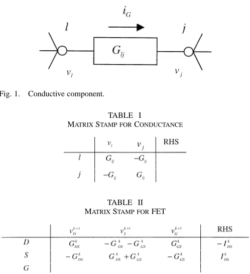
[image:2.612.302.551.58.331.2]Element stamps are small component-specific tables con-taining matrix and excitation data [3]. The table indicates the component values to insert in the nodal admittance matrix and in the RHS vector. For example, consider a linear conductance
Fig. 1. Conductive component.
TABLE I
MATRIXSTAMP FORCONDUCTANCE
TABLE II MATRIXSTAMP FORFET
between two nodes and , with node voltages and , Fig. 1.
This component has the stamp shown in Table I.
It is similarly possible to define stamps for nonlinear ele-ments, and such stamps form an efficient method for updating the admittance matrix and RHS vector. Equation (1) gives the branch current for a field-effect transistor (FET) at the
NR iteration
(1)
where denotes the FET drain-source current at the iteration. The transconductances , , and are the derivatives of with respect to the voltage , where and ( ) can be any of , , or (the drain, the source, and the gate). Note that the above derivation is for the forward bias case of the MOSFET. If the MOSFET goes into reverse bias, then and are swapped. Table II shows the general element stamp for a FET transistor.
The matrix–vector equations can be solved by Gaussian elim-ination or a related algorithm, such as LU factorization. There are other improvements that can be made when we have cer-tain types of matrices. In particular, if a matrix is sparse, one only need store the nonzero entries, thus eliminating unneces-sary calculations [1].
B. The NR Method
The most common method for nonlinear circuit analysis is the NR method coupled with the Gaussian elimination algorithm. We solve the set of nonlinear equations by formu-lating the linearized matrix vector equation (2) using element stamps
Equation (2) is solved to find , the node voltage vector at the iteration. The matrix is the nodal admit-tance matrix, and the RHS vector is the vector of excita-tions. Both are initially set to zero and are updated using el-ement stamps. In fact, to form (2), we need to use the fact that . If we substitute this expression into (2) and
multiply both sides by , we get ,
which is the multidimensional form of the standard
one-dimen-sional Newton formula , where
is the derivative of the device equation with respect to , evaluated at , the th approximation to the root of . By repeatedly solving (2) (using Gaussian elimination or a related technique) and using the solution to formulate the matrix and ex-citation vector for the next iteration, the solution vector should converge to an accurate representation of the state of the circuit. For further reading, the reader is directed to [1]–[3].
This process is computationally intensive. The matrix equa-tion needs to be set up and solved once per Newton iteraequa-tion. Building the Jacobian matrix requires the evaluation of the par-tial derivatives of the device equations. Typically, evaluating the device equations and derivatives, along with the associated ma-trix operations, requires about 70% or more of the total CPU time [4], [5].
C. Convergence
NR has some inherent problems that manifest themselves quite frequently. When they arise, the algorithm can fail to work correctly. One such problem is NR’s sensitivity to the initial values in the solution vector used to start the analysis. This is especially noticeable when we are dealing with nonlinear cir-cuit equations that have multiple solutions. In this case, different initial settings can result in convergence to different solutions or to divergence. In the absence of any other knowledge, the solu-tion vector is initialized to . This may be simplistic because, if there are multiple solutions, they will be missed and the algo-rithm may potentially fail to converge. A randomly initialized set of start points may seem better, but the main reason this is not done is that it may yield more failures than successes or re-peated occurrences of the same solution, all of which increase the running time. There is, however, a technique called
homo-topy which is a more sophisticated approach to this idea [6]–[8],
and which is potentially globally convergent.
The main problem with the selection of the initial values is that one can never be sure of the radius of convergence for a particular problem, and so picking an initial solution that is outside this radius can lead to divergence, or if there are multiple solutions, it could lead to finding a solution other than that being sought. There are several techniques that can be used to help convergence, such as the -coordinate method [2], the error-function-curvature-driven Newton update correction method [9], damping algorithms [10], the source stepping algorithm [11], and the stepping procedure [12].
In 1977, Ho et al. [10] proposed a damping algorithm to aid the convergence of NR. A damping factor is used to aid conver-gence as follows. The damping factor in (3) is initialized to
a small number such that 0 1; is then increased at each iteration until it reaches 1, at which point it remains constant
(3)
The increments of should be quite large for the first few itera-tions but should then decrease gradually. Hence, this technique stops sudden large changes that occur between successive ap-proximate solutions, particularly over the first few iterations.
The stepping procedure aids convergence by adding a constant ( ) onto each diagonal component of the Jacobian matrix . is set to a large initial value and is decreased at each iteration to a value of 10 or less. The constant stops zeros from occurring on the diagonal, which in turn prevents the matrix from becoming singular. This procedure is equivalent to a large resistance (small conductance) being connected between every node in the circuit and ground.
These techniques do not all work for every problem. Hence, commercial simulators employ a number of these techniques and will switch as necessary between them if convergence prob-lems arise. The aim is to develop an EA to find a more general method for solving the majority of circuits.
III. EVOLUTIONARYCOMPUTING
In general, when using EC techniques, for each member of the
population , we aim to optimize and in this case minimize, objectives (nodal equations) for each in-dividual. is the size of the population. Here, represents the th trial vector of node voltages for at the
th generation for . We then form the
ob-jective vector denoted by . We
denote the objectives by , 1, 2, , . For the pur-pose of dc analysis, (the total number of node voltages and branch currents). In the simplest case, contains only node voltages, so we can use these in the evaluation of the de-vice equations. The resulting dede-vice currents can then be used to form the KCL equations for each node. Hence, we define as the net current flowing at node , which is the node’s KCL equation.
device types. Therefore, regardless of which algorithm we em-ploy to find the dc operating points, we can never be sure if there are any solutions left unfound. It is hoped that by the inherent globally convergent properties of EAs, we will find many, if not all, of the solutions when they exist and will not have to rely on user intuition to find the solutions as we do with NR.
A. Fitness Functions
EAs are designed to work on a population of trial vectors and exhibit an implicit parallelism. To enable the processes of evo-lution to be simulated, it is necessary for each member of the population to be assigned a value representing the worth of the solution. This is called the fitness of the individual. The fitness can then be used to decide which trial vectors in the population are to survive from one generation to the next. The general tech-nique is to use and other knowledge about the problem to compute . In the case of dc operating-point analysis, we use the KCL and KVL equations. We use the data in , which is essentially the error vector for , to obtain a fitness score for the trial vector in question. The overall optimization procedure then aims to minimize the fitness scores.
In developing our circuit simulator, we implemented five fit-ness functions but after early investigations, the Euclidean norm was chosen because it provided the best all-round compatibility with the EAs discussed here in terms of convergence times and accuracy. The fitness function is
(4)
B. ESs
ESs are probabilistic heuristic direct-search optimization techniques, invented independently in 1965 by Rechenberg [13] and Schwefel [14]. They operate at the phenotypic level, which has advantages for real-valued problems because there is no need to define suitable genotype representations and the po-tentially complex genotype-to-phenotype mapping functions. There is generally no crossover or inversion in ES [or at least not in the same sense as with genetic algorithms (GAs)], so there is not always a need to find cutting points. Sometimes, however, it can be beneficial to have a crossover-like operator. When this is the case, we use recombination. The cutting points needed for recombination are simpler than those for GA. In ES, cutting points are equivalent to simply deciding which components of the parents’ trial vectors are used to build a recombined intermediate vector . This kind of recombination is called discrete recombination because we are recombining two parents by discretely swapping their vector components, selected at random.
We use a population of size divided into two pools such that , where the first members of the population form the parent pool and the remaining members form the offspring pool. There are several variations of ESs. The first is ( )-ES, where at the end of each generation, the best children are taken as the parents for the next generation for 1 . All other individuals are discarded. Although it can seem like a waste to throw away potentially useful solutions, this form of
ES is known to avoid stagnation. In the developmental stages of this work, the use of this ES was explored but was discarded because it incurred longer running times, and so another form of ES was chosen instead. This version is denoted ( )-ES; at the end of a generation, the best individuals from the union of the parent and offspring pools are taken as the parents for the next generation. Generally, each parent is required to generate at least one offspring. The exact number depends on the value of .
Usually, ESs mutates a parent by adding a Gaussian dis-tributed random vector of mean zero and predefined deviation to it [15] as follows:
(5)
Here, the mutation vector is computed from
(6)
In (6), represents a predefined deviation or step size of the mutation vector at generation , is a user-set scale factor, and is the standard deviation of the th component over the entire population at generation . The new solution has its fit-ness evaluated, and if its fitfit-ness is better than the mean fitfit-ness of the population, then it is included in the offspring pool. This continues until the offspring pool is full.
It can be seen that the basic ES uses the same deviation to generate each variable in all the mutation vectors in a single generation. This is not very realistic because the magnitude of each component of the solution vector can be very different. It can sometimes be better to have a different deviation or step size for each of the components. This can allow for more diver-sity among the solutions and a better exploration of the solution space [15]. If one implemented this directly, it would involve many user-defined parameters; hence, it is useful if the step sizes can self-adapt, thus letting the algorithm find the best settings [16].
One self-adaptive technique is given as follows:
(7)
This provides a different deviation for each variable in . Overall, we form a deviation vector for each trial vector . The variable (0, 1) is a normalized Gaussian random deviate globally set and regenerated at the start of each generation and (0, 1) is the th independent normalized Gaussian random deviate. The parameters and are defined in (8) [16]. is a user-set scale factor
(8)
been mentioned: discrete recombination, but for our ESA al-gorithm, a different recombination operator has been used as a result of earlier experiments. It works as follows. Two parents
vectors and , 1, 2, , are randomly
selected before mutation occurs. The recombined intermediate vector and the intermediate deviation vector are calculated as
(9)
The variable is a uniformly distributed random deviate be-tween 0 and 1. The vector becomes the new offspring , and if its fitness is better than the mean fitness of the population, then it is included in the offspring pool. This continues until the offspring pool is full. When using both mutation and recombi-nation, we first use recombination on the parent pool and then, after generating offspring, we apply mutation to the parent pool and generate further offspring.
C. An EA and Tournament Selection Scheme
The EAs described thus far have had one thing in common, they each use truncation selection [15]. This means that the best individuals are selected from the union of the parent and offspring pools, which become the set of new parents and are ranked in order of fitness. However, with truncation selection, we do not directly have any control over the selection pres-sure on an individual. It has been demonstrated that as selec-tion pressure increases convergence time decreases [15], but in-creasing selection pressure can make it harder to escape from local optima.
Tournament selection is a selection mechanism found in the
area of EC called evolutionary programming [15], [17]. At the start of each generation, each member of the population is, in turn, compared pairwise with each of randomly selected and distinct members of the population, where 1 . For each of the members, a tally point is added onto a temporary tally score , if is fitter than that member. Therefore, any can achieve at most tally points. Hence, we calcu-late the selection probability for as , and so 0 1. When a parent is required, such as in the re-combination or mutation operators, we randomly pick a parent from the population and randomly accept or reject that choice using a coin toss biased according to . We can increase the selection pressure by pitting a parent against more population members, e.g., increasing . Typically, 0.6 , where is the size of the parent pool.
Here, we apply tournament selection to the ES population de-scribed in the previous section. The tournament selection EA (TSEA) uses the mutation operator found in the standard ES and it also uses a recombination operator as used in ESA. The algo-rithm’s operation is the same as ESA, except that we have no parameter self-adaptation and, hence, the deviation vector is no longer required, but mutation and recombination operations are carried out in much the same way. We also do not compare the offspring with the population’s mean fitness before including them in the offspring pool as with ES and ESA. Instead, we just place the first offspring that gets generated, by an operator,
directly into the offspring pool. The only other difference is the need to calculate selection probabilities for each trial solution, as discussed above.
By increasing the selection pressure, we increase the level of discrimination made by the algorithm and hence we get a sub-stantial speed increase. This can have the side effect of making the algorithm find only one out of several possible solutions as can be seen later in the experimental results. If the speed in-crease is sufficient, it is possible to perform multiple runs of the algorithm to find other solutions.
D. Differential Evolution
Storn and Price have described an EA that is self-adaptive, simple, and yet very powerful called differential evolution (DE) [18]. DE is perhaps the simplest EA to implement and to understand out of those described in this paper. It has also been shown [19] to be one of the most robust methods. It has been tested against many other methods, including simulated annealing, adaptive simulated annealing, genetic algorithms, and annealed genetic algorithms, and was found to be at least as good as the other techniques, and in many cases far better.
Several DE schemes have been proposed by Storn [20]; some are more successful than others, and some are problem depen-dent. Only two schemes will be discussed here: DE1 and DE2 [18]. In DE1, for each trial vector in the population, we generate an intermediate vector as follows:
(10)
In (10), is a positive real-valued user-set scale factor and , , and are randomly1 selected integers in the range and are all mutually distinct. The intermediate vector is then used with in a crossover procedure to generate a new
off-spring . If is fitter than , then and
we discard , else we keep . We generate potential off-spring using the following formula:
for
otherwise.
(11) In (11), is a randomly selected integer in the range [0, 1] and is an integer selected from the same range but with the probability , where is the user set crossover probability such that . The notation denotes the
function .
DE2 is identical to DE1 except for the generation of the in-termediate vector . This time, an additional difference vector is used, as follows:
(12)
Note that this time we only need two random integers and , and is positive user-set scale factor. The point of DE2 is that by including the extra difference vector, involving the current generation’s best solution, we enhance the greediness of the algorithm.
1All the random numbers used in DE are assumed to be uniformly distributed
When using DE there are several rules that, where possible, should be obeyed to improve the performance of the algorithm. For instance, it has been suggested that the initial population should be spread over the full range of the problem variables [20]. should usually be set to a value less than 0.5, but if the algorithm fails to converge, then can be increased to as much as 1.0. As an initial guess, the best population size is usually and the user should try [0.5, 1.0]. Further-more, as is increased above 10 , then and should be decreased.
IV. DC ANALYSISUSINGEC
A. Implementation
The new simulator, EACS, has been built on an existing SPICE-like simulator. The existing simulator uses linked lists and similar data structures to represent the circuit components: the circuit nodes and the sparse network matrix. The EC package uses the existing device models to evaluate branch currents (to calculate the fitness of the solution), and returns newly calculated node voltages into the simulator structure. To some extent, therefore, the use of an existing simulator has compromised the performance of the new solution methods, but on the other hand, there are significant advantages to using existing implementations of complex device models.
In addition to NR, the following solution algorithms may be selected: ES, ESA, DE1, DE2, and TSEA. It is possible to man-ually set all relevant scale factors and to choose a fitness func-tion from those discussed in secfunc-tion or to use default settings for each algorithm. As in a conventional SPICE simulator, the set-tings can be applied by setting options in the circuit netlist file. EACS has been tested using a variety of benchmark circuits. A short description of each of these circuits is given in the next subsection and the results of these tests follow.
B. Benchmark Circuits
To test the basic test simulator, several CMOS benchmark cir-cuits were used to evaluate the performance of all of the EAs. SPICE level-3 MOS models were used throughout. Each cir-cuit has one solution, with the inputs described, unless otherwise stated. Circuits such as the latch, the Schmitt trigger, the CMOS inverter, the multiplexers, and the differential pair are often used as benchmark circuits for simulators and the remaining circuits given here are used to test scalability when simulating com-posite circuits, involving subcircuits of devices such as trans-mission gates and inverters. Thus, the benchmark circuits are as follows.
• An inverter containing two MOS transistors, a p-type and an n-type.
• A tristate inverter consisting of four MOS transistors. • An RS latch consisting of two cross-coupled NAND gates
(eight MOSFETs in total). The latch inputs, set (S) and reset (R), were both set at logic 1 (or in analog terms at the supply voltage ). In this mode, the circuit has three possible solutions: 1) output at ; 2) at 0 V; and 3) the metastable state with at approximately /2. This cir-cuit is not difficult to simulate with NR but illustrates NR’s failure to find multiple solutions without the user assistance.
• A transmission gateXORwith inputs 1 and 1. This circuit contains six MOSFETs. The inputs 1 and 0 were also tried but NR failed to converge, while the EAs found the correct solution. NR fails on the second configura-tion due to gain in the circuit and strong positive feedback. • A transmission gate multiplexer (MUX1) consisting of two
transmission gates (four transistors). This circuit should sim-ulate without problem; it is used here to test a composite circuit.
• A tristate inverter multiplexer (MUX2) formed by using tris-tate and regular inverters and consisting of twelve MOS-FETs. This circuit is, again, used to illustrate the use of a larger composite circuit.
• An inverting Schmitt trigger. The Schmitt trigger is made up of five p-type and five n-type MOSFETs. This circuit usually has one solution: the inverse of its input. However, the circuit has hysteresis and when the input voltage is between two critical thresholds the output depends on the previous state of the circuit. In dc analysis, there are two possible solutions as there is no memory of any previous state. This circuit is used to illustrate the failure of NR to find multiple solutions and to show that EAs can be used to simulate a circuit for which NR fails to converge to either solution without user assistance.
• A CMOS differential pair with two nMOS transistors, resis-tive loads, and a constant current source.
• A one-bit adder that is constructed using a transmission gate
XOR(see above) together with two inverters and four trans-mission gates. The three inputs were set to logic 1. The adder contains 18 transistors. Again, this is another composite cir-cuit and is used to test the scalability of our circir-cuit simulator when using EAs.
C. Experimental Results
Five EAs are implemented in the simulator, along with NR. The NR algorithm employs damping in the form of step-size limiting to assist convergence. Initial values can be set to assist convergence.
The following EC algorithms were used for all the benchmark circuits, with the control settings shown.
• DE1: 0.4, 0.5, convergence threshold 5 10 , population size (i.e., number of parents) 10 ( is the number of circuit nodes)
• DE2: 0.8, 0.9, 0.3, convergence threshold
5 10 , 10
• ES: 0.7, Convergence Threshold 5 10 , 50 (“smaller” circuits), 100 (“larger” circuits) • ESA: 1.0, convergence threshold 5 10 ,
150
TABLE III
RESULTS FOR ACMOS NOT GATE(INPUT= 1)
TABLE IV
RESULTS FOR ACMOS TRISTATEINVERTER
TABLE V
RESULTS FOR ACMOS RS LATCH(R = S = 1)
TABLE VI
RESULTS FOR ACMOS XOR GATE(A = B = 1)
by performing several “tune-up” runs of the algorithms across the range of benchmark circuits and these values were found to work well in general. The algorithm halts once the best member of the current population has a fitness less than the threshold.
For the Schmitt trigger and the RS latch, it was necessary to manually set initial conditions to force NR to find all the solu-tions. By default, NR will find the metastable state for the latch. NR will not converge for the Schmitt trigger—it was necessary to artificially set the input voltage just outside the hysteresis band to find a solution.
The performance for each algorithm with each of the cir-cuits is shown in Tables III–XI. The RS latch (Table V) and the Schmitt trigger (Table IX) have multiple solutions. The algo-rithm is stated in the first column of each table. In the second
TABLE VII
RESULTS FOR ACMOS MULTIPLEXER1
TABLE VIII
RESULTS FOR ACMOS MULTIPLEXER2
TABLE IX RESULTS FORSCHMITTTRIGGER
TABLE X
RESULTS FOR ACMOS DIFFERENTIALAMP
TABLE XI
RESULTS FOR ACMOS ONE-BITADDER
Fig. 2. Convergence graph for DE1 and an RS latch.
Fig. 3. Convergence graph for TSEA and an RS latch.
(e.g., 1 1 means two solutions were found by restarting the algorithm). The third column shows the number of generations (or for NR, the number of iterations). The fourth column shows the accuracy compared with the solution found by NR (assumed to be the most accurate). In the case of multiple solutions, the mean error across all solutions is stated. Finally, the CPU time in milliseconds is given. The benchmark tests were run on a PC workstation with an 800-MHz 586 CPU and 256 MB of RAM, running Windows NT. Again, if multiple runs were needed to find multiple solutions, this is stated as a sum. As well as mon-itoring the best solution of the current generation, various other values were monitored at each generation to provide an idea of the performance of the EAs. In particular, the mean fitness, mean solution, and the standard deviation of the population were obtained and stored in a separate results file for later study. This data gives an insight into the convergence of the EAs. Fig. 2 il-lustrates the progression of DE1 for an RS latch, with respect to the mean fitness of the population. (The analysis takes 301 generations, but the graph shows only the first 45 generations.) The initial population’s mean fitness was 5.12 10 and the final population’s mean fitness was 1.08 10 . As another example of the convergence behavior of the EAs, Fig. 3 shows the convergence of TSEA for an RS latch, but unlike DE1, only one solution was found for a single run of TSEA. In this case, the initial population’s mean fitness was 2.50 10 and the final population’s mean fitness was 5.82 10 . A similar pattern can be found among the data collected for the other al-gorithms and circuits.
DE1 and ES are the best algorithms for finding multiple solutions automatically. ESA is least good at finding multiple solutions, even when restarted.
NR is always the fastest, in terms of CPU time (but note the comment above concerning the manual intervention needed to find multiple solutions). For circuits with a single solution, TSEA is always the fastest of the EAs in terms of the number of generations and in terms of CPU time, with the exception of the RS latch, where DE1 is fastest. ESA is consistently the slowest (apart from for the Schmitt trigger circuit, where it only found one solution). The best-performing EAs are, however, between 16 and 170 times slower than NR.
The accuracy of the EAs is very similar. TSEA or DE2 are the most accurate in all cases except MUX1, when ESA is best. It must be noted that all these accuracy figures are relative to NR, and are not absolute errors. The error is calculated as the mean of the difference between the NR solution(s) and the EA solution(s).
In general, therefore, DE1, DE2, ES, and TSEA are accurate and robust in terms of convergence and the number of solu-tions found. Accuracy and speed can be gained at the expense of finding multiple solutions. Although NR is always fast, it may depend on the user setting the initial state of the solu-tion vector. The EAs are more likely to succeed from arbitrary starting points. Therefore, the CPU time does not necessarily represent the total effort required to find a solution. This is par-ticularly true when multiple solutions exist and are sought. It can therefore be argued that the best algorithms in terms of ac-curacy, speed, and the ability to find multiple solutions and to analyze problem circuits, such as the Schmitt trigger, are DE1 and DE2.
V. CONCLUSIONS
The use of EAs for nonlinear operating-point analysis of MOS circuits has been demonstrated. It has been shown that EAs, and particularly DE and TSEA, have some significant advantages over conventional NR. DE and the other EAs are globally convergent, whereas NR is only locally convergent. NR requires manual intervention to find all the solutions to a circuit; it has been shown that DE can find multiple solutions in a single pass. An important property of EAs is that they can find multiple solutions in a single pass, but this can sometimes take significantly longer than using NR to find a single solution. It is important to get a good balance between speed, accuracy, and the number of solutions found. We can often make improvements to an EA that, for instance, increases the speed of the algorithm, but this can have side effects. For example, if we increase the amount of discrimination an algorithm makes with regards to selecting parents, then this gives a speed increase along with improved accuracy, i.e., TSEA. We have seen, however, that there is a significant side effect in losing the ability to find multiple solutions. Hence, if TSEA is to be a suitable alternative to NR, improvements to the algorithm must be made to give it the ability to find all the solutions in a single pass.
recombination strategies, etc. The success of DE is partly due to its self-adaptive nature, and although DE uses mutation as a pri-mary operator, it also contains a recombination operator so as to not neglect the benefits of sexual reproduction. Another excel-lent feature of the DE algorithms is that the population size is au-tomatically scaled in proportion to the size of the given problem, which can help avoid over- and under-sized populations. These features and the way they are implemented in DE have been the major contribution to DE’s good performance.
All of the EAs here are slow compared with NR, even though the Jacobian matrix is not constructed. This can be attributed to two factors. First, a significant amount of sorting of popula-tions has to be done. This accounts for the majority of the CPU time taken. For example, in a -ES, with typical values of 100 and 200, we will have it so the parent pool is or-dered fittest first and the offspring pool is in no particular order. Hence, we will need to reorder a population that may not be close to being correctly ordered and with 300 members, as with the example above; this is not a trivial task. The sorting algo-rithm used, in this version of EACS, is simple and based on the insertion sort. A better choice of algorithm, such as one based on the quick sort algorithm, would produce a significant speed up. Secondly, because the device models have been inherited from an earlier simulator, they evaluate both the current (as required for EC) and the partial derivatives, which are not required. If the models were modified to remove these unnecessary calcu-lations, we would expect the time taken for device evaluation to be approximately halved. Therefore, overall we can reasonably expect that the EAs can be speeded up by at least an order of magnitude. This would make them very competitive with NR. Having demonstrated the computational effectiveness of using evolutionary computation for circuit analysis, the next phase of this research will seek to increase the speed of the algorithms.
As well as increasing the speed, we will also endeavor to improve the accuracy. It is felt that the best way to approach this is by way of a hybrid method with the NR algorithm. In other words, a population can be searched in a fairly coarse way using an EA, perhaps DE1, and then the solution can be refined using NR. This will provide accuracy almost identical to NR and should also reduce the number of generations needed to reach convergence. Much larger benchmark circuits, up to 100 nodes, will be constructed and used to test the performance of the EAs when simulating such large circuits.
ACKNOWLEDGMENT
The authors would like to thank Dr. Z. R. Yang for suggesting the original idea that led to this research.
REFERENCES
[1] V. Litovski and M. Zwolinski, VLSI: Circuit Simulation and
Optimiza-tion. London, U.K.: Chapman and Hall, 1997.
[2] D. A. Calahan, Computer Aided Network Design, revised ed. New York: McGraw-Hill, 1972.
[3] C. W. Ho, A. E. Ruehli, and P. A. Brennan, “The modified nodal ap-proach to network analysis,” IEEE Trans. Circuits and Simulation, vol. CAS-22, pp. 504–509, June 1975.
[4] P. F. Cox, R. G. Burch, D. E. Hocevar, P. Yang, and B. D. Epler, “Di-rect circuit simulation algorithms for parallel processing,” IEEE Trans.
Computer-Aided Design, vol. 10, pp. 714–725, June 1991.
[5] T. A. Johnson and D. J. Zukowski, “Waveform-relaxation-based circuit simulation on the Victor V256 parallel processor,” IBM J. Res. Develop., vol. 35, no. 5/6, Sept./Nov. 1991.
[6] R. C. Melville, L. Trajkovic´, and L. T. Watson, “Artificial parameter homotopy methods for the DC operating point problem,” IEEE Trans.
Computer-Aided Design, vol. 12, pp. 861–877, June 1993.
[7] L. Trajkovic´, “Homotopy methods for computing DC operating points,” School of Eng. Sci., Simon Fraser Univ., Burnaby, BC, Canada, no. 2526, 1996.
[8] D. M. Wolf and S. R. Sanders, “Multiparameter homotopy methods for finding DC operating points of nonlinear circuits,” IEEE Trans. Circuits
Syst. I, vol. 43, pp. 824–838, Oct. 1996.
[9] E. Ngoya, J. Rousset, and J. J. Obregon, “Newton–Raphson iteration speed-up algorithm for the solution of nonlinear circuit equations in general purpose CAD programs,” IEEE Trans. Computer-Aided Design, vol. 16, pp. 638–643, June 1997.
[10] C. W. Ho, D. A. Zien, A. E. Ruehli, and P. A. Brennan, “An algorithm for DC solutions in an experimental general purpose interactive circuit design program,” IEEE Trans. Circuits and Simulation, vol. CAS-24, Aug. 1977.
[11] C. G. Broyden, “A new method of solving nonlinear simultaneous equa-tions,” Comput. J., vol. 12, pp. 94–99, 1969.
[12] T. N. Najibi, “Continuation methods as applied to circuit simulation,”
IEEE Circuits Devices Mag., vol. 5, pp. 48–49, 1989.
[13] I. Rechenberg, Cybernetic Solution Path of an Experimental
Problem. Farnborough, U.K.: Ministry of Aviation, Royal Air-craft Establishment, Aug. 1965, Library Translation no. 1122. [14] H.-P. Schwefel, “Kybernetische Evolution als Stategie der
Experi-mentellen Forschung in der Strömungstechnik,” Diploma thesis, Tech. Univ. Berlin, Berlin, Germany, 1965.
[15] D. B. Fogel, Evolutionary Computation: Toward a New Philosophy of
Machine Intelligence, 2nd ed. New York: IEEE Press, 2000. [16] T. Bäck and H.-P. Schwefel, “An overview of evolutionary algorithms
for parameter optimization,” Evolut. Comput., vol. 1:1, pp. 1–23, 1993. [17] L. J. Fogel, “Autonomous Automata,” Indust. Res., vol. 4, pp. 14–1,
1962.
[18] R. Storn and K. Price, “Differential evolution: A simple and efficient adaptive scheme for global optimization over continuous spaces,” ICSI, Berkeley, CA, Tech. Rep. TR-95-012, 1995.
[19] , “Minimizing the real functions of the ICEC’96 contest by differ-ential evolution,” in Proc. Int. Conf. Evolutionary Computing, Nagoya, Japan, 1996, pp. 842–844.
[20] R. Storn, “On the usage of differential evolution for function optimiza-tion,” ICSI, Berkeley, CA, Tech. Rep., 1996.
Duncan A. Crutchley received the Master’s degree in pure mathematics (with specialization in elliptic curve cryptography) in 1999 from the University of Southampton, Southampton, U.K., in 1999, where he is currently working toward the Ph.D. degree in elec-tronic engineering.
During 1999, he was with Philips Semiconductors, Southampton, U.K. During his time at Philips, he de-veloped elliptic curve cryptosystems for smartcards and IEEE1394 FireWire devices. His research inter-ests are in the area of globally convergent numerical methods for circuit analysis and using such methods to develop a SPICE-like analysis tool. He has published several conference papers on this topic.
Mark Zwolinski (M’92–SM’00) received the B.Sc. and Ph.D. degrees in electronics from the University of Southampton, Southampton, U.K., in 1982 and 1986, respectively.
He is a Senior Lecturer in the Department of Electronics and Computer Science, University of Southampton. His research interests include simulation and modeling algorithms for analog and mixed-signal integrated circuits, fault simulation, high-level synthesis, and test synthesis. He has co-authored over 90 research papers in technical journals and conferences.