A simple approach of determination of the crystallographic orientation: Applications and accuracy

A Simple Approach of Determination of the Crystallographic Orientation: Applications and Accuracy

S.C. Wang* and M.J. Starink

Materials Research Group, School of Engineering Sciences, The University of Southampton, SO17 1BJ, England

Key words: Beam direction, crystallographic orientation, Kikuchi lines

Abstract

A simple analytical solution for the crystallographic orientation has been described. This method is based on one indexed Kikuchi pair in a known zone rather than the corresponding diffraction spots. The accuracy of this method is shown to be better than 0.1º even in the cases where a zone axis is deviated by a large angle (e.g.10º) form the centre of the beam direction. This approach simplifies experiments since only one pair of Kikuchi lines and a zone axis are needed, and is especially suited when it is difficult or cumbersome to resolve a second pair of Kikuchi lines with sufficient accuracy.

1. Introduction

The knowledge of crystallographic orientation is of considerable importance such as in the study of the defects of grains, grain boundaries and heterophase interfaces. Determination of the orientation using TEM has the outstanding advantage that the orientation and image of the microstructure of a specimen can be recorded at the same time with a high spatial resolution. All the accurate methods used to determine the beam direction make use of Kikuchi lines combined with the corresponding diffraction spots. For example, Ryder and Pitsch (1968), Thomas and Goringe (1979) proposed a geometrical method to solve the orientation, in which at least three strong spots and three pairs of Kikuchi lines which were sharp and well defined, not belonging to the same zone were needed in the diffraction pattern. A relatively simple method was proposed by Pumphrey and Bowkett (1970), in

which two Kikuchi bands in addition to the diffraction spots were required. Other methods such as Heimendahl et al (1964), and Ball (1981) make use of at least two or three independent pairs of

Kikuchi lines and diffraction spots. These methods, however, have a similar weakness since the clarity of Kikuchi lines and diffraction spots exist in a slight different range of thickness of a specimen. The convergent-beam-electron-diffraction (CBED) technique, which is available for the modern electron microscopes, may be used to obtain high-quality Kikuchi patterns in a large range of thickness for most specimens. In CBED patterns, however, it may be difficult to identify the correspondence between the Kikuchi lines and diffraction spots as the latter are generally blurred or difficult to resolve. Therefore, application of these methods is limited. To overcome such weakness, Helfmeier and Feller-Kniepmeier (1977) proposed a method based on two pairs of Kikuchi lines without consideration of diffraction spots. This method, however, was found difficult to apply as the signs of two pairs of Kikuchi lines as well as directions of lines perpendicular to the Kikuchi lines must be known.

As the automatic indexing of backscattered Kikuchi bands (BSKB) has already been applied commercially on SEM (e.g. HKL Channel+ software, Oxford Instruments OPAL), a number of recent studies are focused on fully ‘automatic’ indexing of transmission Kikuchi bands (TMKB) on TEM (e.g. Schwarzer 1997, Morawiec 1999 and Zaefferer 2000). The indexing is based on the comparison of measured interplanar angles and interplanar spacings with theoretical values calculated for the actual crystal structure (Schwarzer 1997). However, application of automatic indexing on TMKB is more difficult than on BSKB, because of the generally poorer quality of TMKB, which depends not only the surface strains (similar to BSKB in SEM) but also the specimen thickness. According to Schwarzer (1997), its accuracy by use of automatic indexing was proved up to 0.5º, whereas it is only 0.1º by manual indexing. Thus, manual indexing is still widely used for accurate determination of crystallographic orientations, defect simulations, etc.

In this paper, a new method to determine the beam direction is proposed. There are some advantages in using this method. Firstly, it can be used to analyse patterns which cannot be analysed using other methods, such as patterns where the diffraction spots are blurred or can not be distinguished. Secondly, in general at least one zone and a pair of Kikuchi lines can be recorded in a CBED pattern using a low camera length, thus it is not necessary to search for special orientations where at least two distinct Kikuchi bands can be indexed. It may therefore simplify the procedure to determine the boundary misorientations and heterophase orientation relationships in which usually three pairs of orientations are needed. Thirdly, it can be applied to the case where a zone axis is deviated by a large angle (e.g. 10º) from the beam direction.

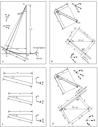
Generally at least one zone can be included in a diffraction pattern recorded using a low camera length. Assuming that the vector parallel to the axis of a zone A is uA and the vector parallel to the beam direction is uO, then a line, which is perpendicular to uA and lies in the plane containing uA and uO, can be obtained. This corresponding vector is designated k. Fig. 1a illustrates the formation of zone A related to the Ewald sphere. O₁ is the centre of the Ewald sphere, O lies on the sphere. uO is parallel to OO₁, and uA is parallel to AO₁. A pair of Kikuchi lines can be formed by the intersection

of the Kossel cones (illustrated by the dotted lines O₁B and O₁C in two dimension) and the Ewald

sphere. B and C are the positions of a pair of Kikuchi lines viewed end-on, and A is the central

position. The distance of the Kikuchi band away from the beam centre recorded in the plane perpendicular to uO is A₂O, and the corresponding distance in the plane perpendicular to uA is AO₂.

Assuming that in reciprocal space AO₂ = m, A₂O = and AO₁ = OO₁ = 1/λ (where λ is the electron

wave length), then the following equation is obeyed ' m

( )

( )

k

k

u u

u ⋅

⋅ λ +

⋅ λ − ⋅ ⋅ λ + =

m m

m A 2

A 2 O

1 1

1

(1)

The top diagram in Fig. 1b shows the relations among g, k2 and k in the plane perpendicular to uA, as

seen from Fig. 1a, the distance of AO2is m, thus,

k k g

g k

2 2

⋅ + + ⋅ + =

m m

m m

m m

2 2 2 1

2 2

2 2 1

1

(2)

where g is a reciprocal lattice vector perpendicular to a pair of Kikuchi lines which lie perpendicular to uA, and k2 is the vector parallel to a line which lies perpendicular to g and uA, m1 and m2 are the components of m resolved parallel to g and k2, respectively, then

k2 = g× uA (3)

Combining equations (1~3), the beam direction can be solved if m₁, m₂and m are known. However,

these data cannot be obtained directly because TEM measurements are carried out on the plane perpendicular to uO rather than on the plane perpendicular to uA.

If k' and m' represent the projected direction and distance in the plane perpendicular to uO

corresponding to k and m in the plane perpendicular to uA, then the following relation is satisfied

from Fig. 1a,

( )

m m m

' '

⋅ λ − =

2

1

(4a)

where ψ is a angle between uOand uA or between k and k'.

Similarly, if and are vectors parallel to the projections of g and k₂, respectively, perpendicular to uO and having magnitudes and m , respectively, then the angles ψ1 and ψ2 corresponding to

g^ and k₂^ , respectively (see Fig. 1c), are given by 1

'

k k'2

m'1 '2

1 '

k k'2

( )

m m m

' 1 ' 1 1

⋅ λ − =

2

and

( )

m m m ' 2 ' 2 2 ⋅ λ − = 2 1 (4c)

It is worth noting that although g is perpendicular to k₂ in the plane normal to uA, it does not mean that their projected lines and in the plane perpendicular to uO are still perpendicular. The bottom of Fig. 1b illustrates the relation between and in the plane perpendicular to uO. Thus, and cannot be obtained directly from a CBED pattern unless φ is known. As shown in Fig. 1b, only the components ∆₁ and ∆₂ (perpendicular to and parallel to the projected Kikuchi lines) can be given. Their relations are as follows

1 '

k k'2

1 '

k k'2

m'1 m'2

( )

φ ⋅ λ ⋅ Δ = sin 1 L

m'1 (5a)

( )

λ ⋅ φ Δ − Δ = L m'2

tan c

1

2 _(5b)

and

( ) ( )

λ ⋅ Δ + Δ L =

m' 2

2

12 _(5c)

where L is the effective camera length. From the appendix, φ may be given by equation (A5), then

1 '

m and m2' can be expressed by ∆1 and ∆2.

With the above procedure, once the experimental measurements of ∆1, ∆2 and the effective camera

length L are obtained, the beam direction can be calculated,

_{( ) ( )}

⎟ ⎟ ⎠ ⎞ ⎜ ⎜ ⎝ ⎛ + + + − Δ + Δ − = k k g g u u u 2 2 n 1 2 2 12 2 A A 0 1 1 n 1 1 1 1 L (6) where

( ) ( )

( )

(

( )

)

(

( )

)

_{( )}

(

_{( ) ( ) ( )}

( ) ( )

)

_⎟⎟⎟ ⎟ ⎠ ⎞ ⎜ ⎜ ⎜ ⎜ ⎝ ⎛ − ⎟ ⎠ ⎞ ⎜ ⎝

⎛ _{⋅ − Δ − Δ + Δ} ⋅ Δ Δ − Δ − ⋅ ⎟ ⎟ ⎠ ⎞ ⎜ ⎜ ⎝ ⎛ − Δ − ⋅ Δ − ⋅ Δ Δ − Δ − ⋅

= ( ) 1 1

n 12 2 2 12 2 2 2 2 2 2 12 2 4 22 2 12 2 12 2 2 12 2 4 L L L L L L L L

The equation (6) gives the resolution for the beam direction. However, the equation for factor n is very complex and possible measurement errors introduced are, therefore, not easy to be determined. However if ∆₁=0, then equation (6) can be simplified as

_{( )}

k k u u u 2 2 22 2 A A 0 1 1 _⋅ − Δ − = L (7) Then k k g g 2 2 2 1 Δ

Δ ⋅ + ⋅ and

_{( ) ( )}

Δ

( ) ( )

k k g

g

k k g

g

u u u

2 2 2 1

2 2 2 1

2 2 12

2 A

A 0

Δ Δ

Δ Δ

1

Δ Δ

1

⋅ + ⋅

⋅ + ⋅ ⋅ − +

− =

L

(8)

where k2 = g× uA in case of Fig. 1b (8a)

or k2 = uA× g in case of Fig.1d (8b)

Equation (8) has also been proven, experimentally, to given the same resolution as equation (6) (Wang 1998).

3. Applications and Accuracy

To resolve the beam direction in Equation (8), five steps are suggested to follow: (1) experimental measurements of ∆₁, ∆₂; (2) determination of the zone axis uA based on the diffraction or Kikuchi pattern; (3) determination of one Kikuchi band g; (4) choice of direction k2 by drawing a direction

line from the known zone to the required zones/ beam centre; (5) calculation of the effective camera length L. There are two approaches to determine L: one is L = R⋅d/λ, where R is distance between one

pair of Kikuchi lines in reciprocal space and d is the spacing of the corresponding plane. The second

is L = ∆/sinϕ, where ∆ and ϕ are distance and angle between two known zones. It is recommended

to use the second method if more than two zones of Kikuchi patterns are recorded.

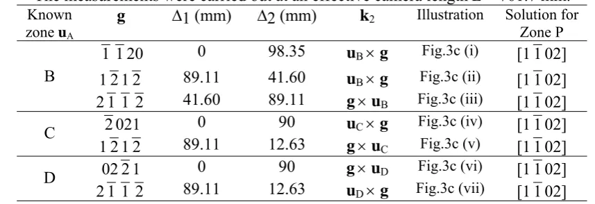
[image:5.595.81.503.88.194.2]

The validity of this method can be confirmed by analysing patterns obtained at orientations where three or more zone axes were recorded using TEM. Fig. 2a shows an example of such a CBED pattern from hexagonal Ti: the arrow indicates the centre of electron beam. Fig. 2b shows the schematic diagram of Fig. 2a. Four zone axes were determined as: Zone B, [2 2 03]; Zone C, [7,8 ,1,12], Zone D, [8, 7 , 1 ,12] and Zone P, [1 1 02]. Assuming that the lattice parameters are a = 0.29511 nm, c = 0.46843 nm, the angle between B, C, and D away from P are calculated: ϕBP = 7.418º, ϕCP = 6.785º and ϕDP = 6.785º. The effective camera length is 761.7(4) mm, and hence the distances between two zones are: ∆BP = L sin(ϕBP) = 98.35 mm; ∆CP = L sin(ϕCP) = 90 mm; ∆DP = L sin(ϕDP) = 90 mm. Fig. 3c and the column 5 in Table 1 show the relations among uA (=uB, uC or uD), g and k2. When these data were input in equation (8) and all the solutions for zone P gave uP = [1 1 02] (see Table 1 for detail), which clearly proved the validity of equation (8).

Table 1. Calculation of zone axis P from equations (8) based on different g and known zone axes. The measurements were carried out at an effective camera length L = 761.7 mm.

Known zone uA

g ∆_{1 (mm)} ∆_{2 (mm)} k2 Illustration Solution for

Zone P

1 1 20 0 98.35 uB× g Fig.3c (i) [1 1 02] 1 2 1 2 89.11 41.60 uB× g Fig.3c (ii) [1 1 02] B

2 1 1 2 41.60 89.11 g× uB Fig.3c (iii) [1 1 02]

2 021 0 90 uC× g Fig.3c (iv) [1 1 02]

C

1 2 1 2 89.11 12.63 g× uC Fig.3c (v) [1 1 02] 02 2 1 0 90 g× uD Fig.3c (vi) [1 1 02] D

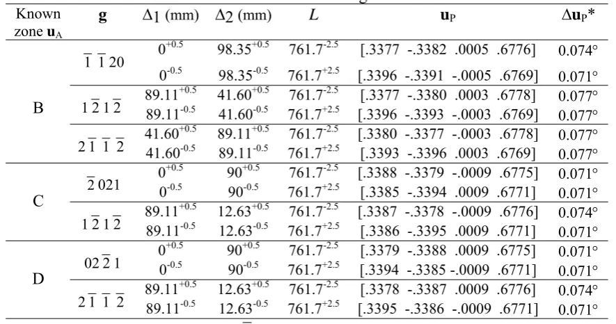
[image:5.595.83.512.602.749.2]

The error for solution of the direction in equation (8) may be estimated by assuming that the maximum errors by experimental measurements of ∆1, ∆2 are ±0.5 mm and the error for the effective

camera length L is ±2.5mm. As shown in equation (8), ∆₁ and ∆₂ have the opposite effects on uO compared to L, thus opposite values are chosen. The details are shown in Table 2, which indicates

[image:6.595.80.523.240.473.2]

that the maximum errors are indeed less than 0.1º. Similarly, a lot of data are available to solve the beam direction of spot O as shown in Table 3. The resultant uO are very close to each other and the remaining small deviations (less than 0.03º) are believed to be caused by the measurements.

Table 2. Zone axes and the beam direction calculated by equations (8). The measurements were carried out at an effective camera length L = 761.7±2.5 mm.

Known zone uA

g ∆₁ (mm) ∆₂ (mm) L uP ∆uP*

0+0.5 _98.35+0.5 _761.7-2.5 _{[.3377 -.3382 .0005 .6776] 0.074°}

1 120

0-0.5 _98.35-0.5 _761.7+2.5 _{[.3396 -.3391 -.0005 .6769] 0.071°}

89.11+0.5 _41.60+0.5 _761.7-2.5 _{[.3377 -.3380 .0003 .6778] 0.077°}

1 2 1 2 _89.11-0.5 _41.60-0.5 _761.7+2.5 _{[.3396 -.3393 -.0003 .6769] 0.077°}

41.60+0.5 _89.11+0.5 _761.7-2.5 _{[.3380 -.3377 -.0003 .6778] 0.077°}

B

2 1 1 2 _41.60-0.5 _89.11-0.5 _761.7+2.5 _{[.3393 -.3396 .0003 .6769] 0.077°}

0+0.5 ₉₀+0.5 _761.7-2.5 _{[.3388 -.3379 -.0009 .6775] 0.071°}

2021 ₀-0.5 ₉₀-0.5 _761.7+2.5 _{[.3385 -.3394 .0009 .6771] 0.071°}

89.11+0.5 _12.63+0.5 _761.7-2.5 _{[.3387 -.3378 -.0009 .6776] 0.074°}

C

1 2 1 2 _89.11-0.5 _12.63-0.5 _761.7+2.5 _{[.3386 -.3395 .0009 .6771]}

0.071°

0+0.5 90+0.5 761.7-2.5 [.3379 -.3388 .0009 .6775] 0.071°

02 2 1 ₀-0.5 ₉₀-0.5 _761.7+2.5 _{[.3394 -.3385 -.0009 .6771]}

0.071°

89.11+0.5 12.63+0.5 761.7-2.5 [.3378 -.3387 .0009 .6776] 0.074°

D

2 1 1 2 89.11-0.5 _12.63-0.5 _761.7+2.5 _{[.3395 -.3386 -.0009 .6771] 0.071°}

* The deviation of the calculated uP from [1 1 0 2]

Table 3. Zone axes and the beam direction calculated by equations (8). The measurements were carried out at an effective camera length L = 760 mm.

Known zone uA

g ∆1 (mm) ∆2 (mm) k2 u0 ∆u0*

1 1 20 1 47.5 _{uB× g} [.3802 -.3786 -.0016 .6511] 0.03º 1 2 1 2 43.5 19 _{uB× g} [.3801 -.3788 -.0013 .6511] 0.03º

B

2 1 1 2 42 21 _{g× uB} [.3805 -.3792 -.0013 .6508] 0.02º 2021 29.5 48 _{uB× g} [.3806 -.3788 -.0018 .6509] 0.02º

C

1 2 1 2 43.5 36 g× uB [.3806 -.3787 -.0019 .6509] 0.03º

02 2 1 27 46 g× uB [.3808 -.3791 -.0017 .6507] 0.03º D

2 1 1 2 42 33.5 _{uB× g} [.3805 -.3793 -.0012 .6508] 0.02º * The deviation of uO from the mean direction which is [0.3805 -0.3790 -0.0015 0.6509]

[image:6.595.78.523.540.682.2]

Firstly, it can be used to analyse patterns which cannot be analysed using other methods. For example, Fig. 3 shows a CBED pattern near [2 4 23] zone of Ti5Si3 phase with only one pair of

Kikuchi lines resolved. No published approaches can be used easily to solve the beam direction in this case since the corresponding diffraction spots are difficult to distinguish. However, it is easy to determine the beam direction using our method. Assuming that the lattice parameters of Ti₅Si₃ are a

= 0.7444 nm, c = 0.5143 nm, the beam is O indicated by the needle. At the effective camera length L

= 440 mm, ∆_{1 and} ∆_{2 were measured to be 18.5 and 1 mm, respectively. As the pair of Kikuchi lines}

relative to the beam direction in Fig.3 are similar to Fig.1b, i.e. k₂ = g× uA, then the beam direction was calculated as [0.4156 -0.7717 0.3561 0.5745] using equation (8) (g = 1 010, uA=[2 4 23]). The new method has been developed especially for the determination of boundary misorientations from pairs of diffraction patterns where it is usually difficult to have both patterns aligned to contain the two zones of spots which are necessary for the subsequent analysis. This method is also convenient for determination of the foil normal which may deviate far from the zone axis which can be indexed, and for the computer simulation of defects in two beam conditions where in general the beam is 5-10˚ away from the low indexed zone. This method has been presented in hexagonal crystals and may apply to any other systems.

4. Conclusion

A simple analytical solution (equation 8) for the electron beam has been devised. This solution is based on only one indexed Kikuchi pair in a known zone, disregard of the corresponding diffraction spots. The accuracy of the method is shown experimentally to be better than 0.1˚ in the cases where a zone axis is deviated by up to 10˚ from the centre of the beam direction, which is comparable to the accuracy of other published methods. Such errors are caused by the experimental measurements rather than by this approach.

ACKNOWLEDGEMENTS

The authors are grateful to Prof. M Aindow at University of Connecticut for helpful discussions.

References

Ball, C.J. (1981) Accurate determination of crystallographic orientation from Kikuchi pattern. Phil. Mag. A, 44, 1307-1317

von. Heimendahl M., Bell, W. and Thomas, G. (1964) Applications of Kikuchi line analyses in electron microscopy. J. Applied Physics, 35, 3614-3616

Helfmeier, H. and Feller-Kniepmeier, M. (1977) Analytical determination of the exact primary beam direction from Kikuchi patterns, J. Applied Physics, 48, 3997-3997

Morawiec, A. (1999) Automatic orientation determination from Kikuchi patterns. J. Appl. Cryst. 32, 788-798 Pumphrey, P.H. and Bowkett, K.M. (1970) An accurate method for determining crystallographic orientations

by electron diffraction. Phys. Stat. Sol. A, 2, 339-346

Ryder, P.L. and Pitsch, W. (1968) On the accuracy of orientation determination by selected area electron diffraction. Phil. Mag. A 18, 807-816

Schwarzer, R.A. (1997) Advances in crystal orientation mapping with the SEM and TEM. Ultramicroscopy, 67, 19-24

Thomas, G. and Goringe M.J. (1979) Transmission electron microscopy of materials. New York

Wang, S.C. (1998) High angle grain boundary structure in Widmanstätten alfa Ti microstructures. PhD thesis, University of Birmingham

k' k Screen Ewald Sphere A O O

u _uA

m' ψ 1/λ 1 O 2 A A1 2 O m B C 2θΒ • • • a

A p_air of Kik

uch i lin_es

φ

2

Δ Δ1

O 1 ' k ' k

⋅'1

m Lλ

[image:8.595.82.491.90.620.2]

⋅m' Lλ ⋅ 2' m L_λ 2 A 2 ' k φ 90º g k k2 m 90 ° m1 m2 A O2 • uA b m ' m ψ O u k k' 2 m 2' m ψ O u g O u k ψ m' m 2 2' k 2 1 ' k 1 1 1 d c

Fig. 1a A schematic diagram showing the geometry of Ewald sphere

Fig. 1b The top schematic diagram showing the relationship of g, k and k2 (k2 = g×uA) in the plane

perpendicular to uA and the bottom one showing the projected lines in the plane perpendicular to uO

Fig. 1c Concise diagram shows the relations of dislocations in the planes perpendicular to uO and uA

Fig. 1d similar to 1b, but k2 = uA×g

A pa ir of

Kiku chi li

nes

φ ⋅ O

' m Lλ 1 ' k 2 ' k ' k ⋅ 1 ' m L_λ

⋅_m'2

P B

C D

O ] 03 2 2 [

] 12 , 1 , 7 , 8 [

] 02 1 1 [

20 1 1 2

1 1 2

] 12 , 1 , 8 , 7 [

b

2 1 2 1

021 2 1

2 02

a

P

•

uB

g

k2/k

•

g

k k2

uB

uB

•

g k

k2

c

•

g uC

k2/k

uC

•

g k

k2

•

g k

k2

uD

• g

uD

k2/k

[image:9.595.55.487.93.479.2]

i ii iii iv _v vi vii

Fig. 2 The CBED pattern and the corresponding schematic program near [1 1 02] of hexagonal titanium. (a) the recorded Kikuchi pattern; (b) illustration diagram

•

uA g

k k2

[image:11.595.46.511.68.769.2]

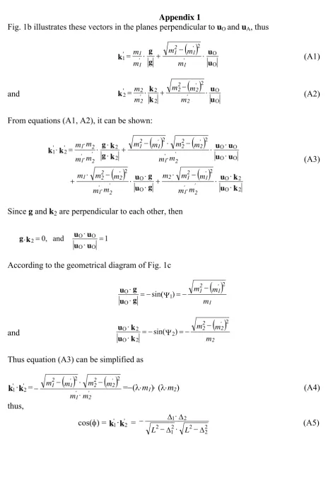
Appendix 1

Fig. 1b illustrates these vectors in the planes perpendicular to uOand uA, thus

( )

u u g g k O O 2 ' 1 ⋅ − + ⋅ = m m m m m ' 1 ' 1 2 1 ' 1

1 _(A1)

and

( )

u u k k k O O 2 2 2 ' 2 ⋅ − + ⋅ = m m m m m ' 2 ' 2 2 2 ' 2 2 (A2)

From equations (A1, A2), it can be shown:

( )

( )

( )

( )

k u k u g u g u u u u u k g k g k k 2 O 2 O 2 O O 2 O O O O 2 2 2 2 ' 2 ' 1 ⋅ ⋅ ⋅ ⋅ − ⋅ + ⋅ ⋅ ⋅ ⋅ − ⋅ + ⋅ ⋅ ⋅ ⋅ − ⋅ − + ⋅ ⋅ ⋅ ⋅ ⋅ = ⋅ m m m m m m m m m m m m m m m m m m m m ' 1 ' 2 ' 1 2 1 2 ' 1 ' 2 ' 2 2 2 1 ' 1 ' 2 ' 2 2 2 ' 1 2 1 ' 1 ' 2 1 2 (A3) Sin

ce g and k2 are perpendicular to each other, then

1 and

,

0 O O

2 =

⋅ =

⋅k u u

g

O O⋅u

u

According to the geometrical diagram of Fig. 1c

( )

m m m 1 ' 1 2 1 2 1 O

O _{sin( )=−} −

Ψ − = ⋅ ⋅ g u g u

and

( )

m m m 2 ' 2 2 2 2 2 2 O 2

O _{=−sin(Ψ )=−} −

⋅ ⋅ k u k u

Thus equation (A3) can be simplified as

1 '

k ·k'2=

( )

( )

m m m m m m ' 2 ' 1 ' 2 2 2 ' 1 2 1 ⋅ − ⋅ − − 2 2

=−(λ⋅m1)⋅ (λ⋅m2) (A4)

thus,

cos(φ) = ·k1' k'2 =

Δ − ⋅ Δ − Δ ⋅ Δ − 2 2 2 2 1 2 2 1 L

L (A5)