Fast Gait Parameter Estimation for
Frontal View Gait Video Data Based on the Model
Selection and Parameter Optimization Approach
Kosuke Okusa and Toshinari Kamakura
Abstract—We study the problem of analyzing and classifying frontal view gait video data. In this study, we focus on the human walking speed and amplitude of arm swing and leg swing, we estimate these parameters using the statistical registration and modeling on a video data. To demonstrate the effectiveness of our method, we apply our gait parameter estimation model for the human gait video data. As a result, our model is able to estimate the gait parameters by stably at low calculation cost.
Index Terms—Gait analysis, human gait modeling, parameter selection.
I. INTRODUCTION
W
E study the problem of analyzing and classifying frontal view gait video data. A study on the hu-man gait analysis is very important in the fields of the health/sports management, medical research.Gait analysis is mainly based on motion capture system and video data. The motion capture system can give the precise measurements of trajectories of moving objects, but it requires the laboratory environments and we cannot be used this system in the field study. On the other hand, the video camera is handy to observe the gait motion in the field study. From the standpoint of health/medical research area. Gage [1] proposed brain paralysis gait analysis using gait video data. Kadabaet al.[2] discussed importance of lower limb in the human gait using gait video data too. Many gait analysis have recently analyzing using video analysis software (e.g. Dartfish, Contemplas, Silicon Coach). For example, Borelet al. [3] and Gruntet al. [4] proposed infantile paralysis gait analysis using lateral view gait video data.
On the other hand, from the standpoint of statistics, Olshen et al. [5] proposed the bootstrap estimation for confidence intervals of the functional data with application to the gait cycle data observed by the motion capture system.
However, most studies have not focused on frontal view gait analysis, because such data has many restrictions on analysis based on the filming conditions.
The video data filmed from the frontal view is difficult to analyze, because the subject getting close in to the camera, and data includes the scale-changing parameters [7], [8]. To cope with this, Okusaet al.[9] and Okusa & Kamakura [10] proposed a registration for scales of moving object using the method of nonlinear least squares, but Okusa et al.[9] and
This research is supported by the Institute of Science and Engineering of Chuo University.
K. Okusa is with the Department of Science and Engineering, Chuo University, Tokyo, 1128551 Japan e-mail: [email protected].
T. Kamakura is with the Department of Science and Engineering, Chuo University, Tokyo, 1128551 Japan e-mail: [email protected].
Okusa & Kamakura [10] did not focus on the human leg swing.
Okusa & Kamakura [12] focus on the gait analysis using arm and leg swing model with estimated parameters and application to the normal/abnormal gait analysis. However, their models have many of parameters, and it raise calculation cost and instability of parameter estimation.
Okusa & Kamakura [13] focus on the calculation cost and parameter estimation stability. The performance of Okusa & Kamakura [13] model is able to speed up the parameter estimation. However, the problem of parameter estimation stability still remains to be solved.
In this study, from the stand point of stability of parameter estimation, we suppose that important gait parameters are walking speed and amplitude of arm swing and leg swing, we redesign the frontal view human gait model. To demonstrate the effectiveness of our method, we apply our gait parameter estimation model for the human gait video data.
As a result, our model is able to estimate the gait param-eters stably at low calculation cost.
II. FRONTALVIEWGAITDATA
In this section, we describe an overview of frontal view gait data. Many of gait analysis using lateral view gait data, because lateral view gait is easy to detect the human gait features. However, in a corridor like structure, the subject is approaching a camera. Such case is difficult observe lateral view gait.
In a lateral view gait, at least two cycles or four steps are needed. For more robust estimation of the period of walking, about 8m is recommended. To capture this movement, the camera distance required is about 9m. Practically, having such a wide space is difficult. On the other hand, frontal view gait video is easy to observe 8m (or more) gait steps [8].
Figure 1 is an example of frontal view gait data recorded by Figure 2 situation. Figure 1 illustrates difficulty of frontal view gait analysis. Even if subject do the same motion with the same timing, frontal view gait data includes scale changing components. Figure 3 shows subject’s width time-series behavior of frontal view gait data. This figure illus-trates frontal view gait data contains many of time-series components.
IAENG International Journal of Applied Mathematics, 43:4, IJAM_43_4_08
Fig. 1. Frontal view gait data
Fig. 2. Filming situation of frontal view gait data
0 1 2 3 4 5
60
80
100
120
140
Time
Width (pixel)
Fig. 3. Time-series behavior of frontal view subject width
III. MODELING OF FRONTAL VIEW GAIT DATA
A. Preprocessing
The raw video data is difficult to observe subject width and height time-series behavior, because data contains back-ground. We separate subject from background using inter-frame subtraction method (Eq. 1).
∆(T)=|I(T+1)−I(T)|, T = 1, ...,(n−1),
∆(T)(p, q) = {
1 (∆(T)(p, q)>0)
0 (Otherwise). (1)
Here, ∆(T) is an inter-frame subtraction image, I(T) is grey scaled video data image at frameT,(p, q)is the pixel coordinate.
a) Subject Width/Height Calculation: Inter-frame sub-traction method can separate the subject and background. However, it is difficult to measure the time-series behavior of the subject width and height. In this section, we describe the subject width and height calculation method using inter-frame subtraction data.
Let us suppose that inter-frame subtraction image is binary matrix. We can measure the subject height and width by integration calculation of row and column at each frame. In this study, we focus on the human gait arm and leg swing of the frontal view gait. We assume that subject width and height time-series behavior consist of the arm and leg swing behavior.
[image:2.595.65.262.167.285.2]B. Relationship between camera and subject
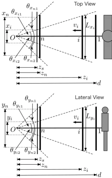
Figure 4 shows a relationship between camera and sub-ject. From figure 4, Width and height modeling has same structure. In this section, we describe the subject’s width modeling. We can assume simple camera structure. We consider the virtual screen exists between observation point and subject, and we definexi as subject width on the virtual
screen ati-th frame (i= 1, ..., n).
i
1
O
v
iz
sz
nz
id
n
x
ix
ni
1
O
v
iz
sz
nz
id
n
y
iy
nTop View
Lateral View
L
xiL
yiθ
xi1
θ
xi2
θ
xn2θ
xn1
θ
yi1
θ
yi2
θ
yn2θ
yn1
Fig. 4. Relationship between camera and subject
Here we define zi, zj as distance between observation
point and subject ati-th, j-th frame,zsas distance between
observation point and virtual screen, θxi1, θxi2 as subject
angle of view from observation point at i-th frame, d as distance between observation point and 1st frame, vi as
subject speed at i-th frame. Okusa et al. [9] defined the subject length L was constant. We assume that L has the time-series behavior and we defineLi is the subject length
ati-th frame.
IAENG International Journal of Applied Mathematics, 43:4, IJAM_43_4_08
[image:2.595.325.517.341.645.2] [image:2.595.63.264.356.544.2]xi ati-th frame depends onθxi1,θxi2 as shown in Figure
4.
xi=zs(tanθxi1+ tanθxi2). (2)
Similarly, the subject length at i-th frame is
Lxi =zi(tanθxi1+ tanθxi2). (3)
From Eq.(2), Eq.(3), ratio between xn andxi is
xn
xi
= Lxnzi
Lxizn
(4)
Frame interval is equally-spaced (15 fps). Okusaet al.[9] assumed the average speed is constant. We can assume that average speed from i-th frame is (n−i) = (zi−zn)/¯v ,
thereforeziiszi=zn+ ¯v(n−i). We substitutezi to Eq.(4)
xi=
Mxiγ
γ+ (n−i)xn+i, (5)
whereγis zn/v¯,Mxi is Lxi/Lxn,iis noise. From Eq.(5),
predicted value xˆ(in) is registration from i-th frame’s scale ton-th frame’s scale
ˆ
x(in)= γ+ (n−i)
Mxiγ
xi. (6)
Similarly, we can define subject height as
yi=
Myiγ
γ+ (n−i)yn+i, (7)
whereMyi is Lyi/Lyn.
Next, we discuss the scale changing, human movement, and speed changing parameter estimation model.
C. Scale changing parameter estimation
From Eq.(5), scale parameter is γ. Solve Eq.(5) for γ
shows
γ= xi(n−i)
xi−Mxixn
. (8)
Here γ is the ungaugeable parameter, and we estimate it using nonlinear least squares method
S(γ, Mxi) =
n
∑
i=1
{
xi−
Mxiγ
γ+ (n−i)xn
}2
. (9)
D. Human movement parameter estimation
Mxi andMyi are movement model of the subject. If the
subject is the rigid body, movement modelMxi andMyi are
constant. Meanwhile, human gait is not a constant.Mxi and Myi needs the movement model because the subject body is
moving wildly.
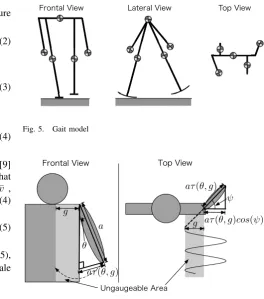
b) Human gait modeling: arm swing: Collinset al.[14] has reported that arm swing is an very important role in the gait motion. We consider the human gait model based on Collins et al.[14] model (see Figure 5).
[image:3.595.45.547.47.464.2]Frontal View Lateral View Top View
Fig. 5. Gait model
θ
g
Ungaugeable Area
Frontal View Top View
aτ(θ, g)
aτ(θ, g)
ψ g
a aτ(θ, g)cos(ψ)
Fig. 6. Arm swing model
It seems reasonable to think that arm swing is single pendulum. Collinset al.[14] model assumed that arm swing is move to anteroposterior direction. Our model, on the other hand, can assume that arm swing move to an oblique direction (Figure 6).
Figure 6’s model has an ungaugeable area. Our method’s width/height calculation is based on integration calculation of row and column at each frame. If the arm move to inside the body area, arm length is ungaugeable. Arm swing model is
xi=
(
W(P1,P2,Q1,Q2,g1,g2,f,i)
W(P1,P2,Q1,Q2,g1,g2,f,n)+s
)
γ
γ+ (n−i) xn+i
W(P1, P2, Q1, Q2, g1, g2, f, i) =
P1τ(f i+Q1, g1) +P2τ(f i+Q2, g2)
τ(θ, g) =
{
sin(θ) +g (sin(θ) +g >0)
0 (Otherwise) (10)
where P1 = a1cos(ψ) and P2 = a2cos(ψ). P1τ(f i+
Q1, g1)andP2τ(f i+Q2, g2) are right and left arm model respectively. From Eq.(10), we estimate each gait parameter using nonlinear least squares method.
S(γ, P1, P2, Q1, Q2, g1, g2, f, s) =
n
∑
i=1
{
xi−
(
W(P1,P2,Q1,Q2,g1,g2,f,i)
W(P1,P2,Q1,Q2,g1,g2,f,n)+s
)
γ
γ+ (n−i) xn
}2
(11)
Here,f is gait cycle frequency,sis adjustment parameter,
P1, P2 are arm swing amplitude parameters,Q1, Q2are arm phase parameters, andg1, g2 are ungaugeable area parame-ters.
IAENG International Journal of Applied Mathematics, 43:4, IJAM_43_4_08
[image:3.595.281.546.49.349.2]c) Human gait modeling: leg swing: Leg swing mod-eling is simpler than arm swing model because leg swing model does not have a ungaugeable area. Okusaet al.[9] and Okusa & Kamakura [10] does not consider the leg swing. It seems reasonable to think like arm swing that leg swing is single pendulum (Figure 7).
bcos(ω)
ω
[image:4.595.307.546.51.253.2]b
Fig. 7. Leg swing model
Leg swing model is
yi=
(
H(b1,Q3,f,i)
H(b1,Q3,f,n)+s
)
γ
γ+ (n−i) yn+i
H(b1, Q3, f, i) =b1cos(f i+Q3). (12)
Here b1 is leg swing amplitude parameter, andQ3 is leg phase parameter.
E. Speed changing parameter estimation
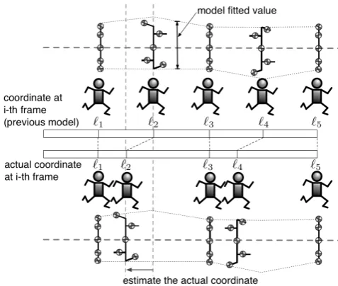
Frontal view video data is difficult to see the subject’s speed. If our gait model is correct, observed valuexiandyi
is same as the fitted value of gait model at point`i. Previous
model’s `i assumes equally spaced (`i =i = 1, ..., n). We
estimate `xi and`yi value for minimize the observed value
and model fitted value at `i. We can define estimated value `xi and`yias a virtual space coordinate at i-th frame (Figure
8).
Eq.5, Eq.7 with the coordinate estimation shows
xi =
Mxiγ
γ+ (n−`xi)
xn+i
yi=
Myiγ
γ+ (n−`yi)
yn+i. (13)
Here, `xi, ..., `xn and `yi, ..., `yn are virtual space
coor-dinate parameters of width and height respectively. From Eq.13, arm swing and leg swing model with the coordinate estimation shows Eq.14, Eq.15.
xi=
(W(P1,P2,Q1,Q2,g1,g2,f,`
xi)
W(P1,P2,Q1,Q2,g1,g2,f,`xn)+s
)
γ
γ+ (n−`xi)
xn+i
W(P1, P2, Q1, Q2, g1, g2, f, `xi) =
P1τ(f `xi+Q1, g1) +P2τ(f `xi+Q2, g2)
τ(θ, g) =
{
sin(θ) +g (sin(θ) +g >0)
0 (Otherwise). (14)
yi=
(H(b
1,Q3,f,`yi)
H(b1,Q3,f,`yn)+s
)
γ
γ+ (n−`yi)
yn+i
[image:4.595.47.284.136.346.2]H(b1, Q3, f, `yi) =b1cos(f `yi+Q3). (15)
Fig. 8. Virtual space coordinate estimation
We suppose that virtual space coordinate of subject is ˆ
`i= (ˆ`xi+ ˆ`yi)/2. Then, we can assume that subjects speed
is 1st order difference of `ˆi, and acceleration is 2nd order
difference of`ˆi.
IV. EFFECTIVENESS OF EACH PARAMETERS
In this section, we discuss the effectiveness of each pa-rameters. From the standpoint of gait analysis, we think the subject’s parameter stability is most important factor.
Eq.14 and Eq.15 models has many of parameters, we need to estimate n+ 11 parameters. It raise calculation cost and instability of parameter estimation.
To cope with this, we confirm the most affected param-eters. We choose 30 subjects and calculate the interclass stability index C for each estimated parameters. Parameter
k’s interclass stabilityCk calculation is
Ck=
∑
p6=q|Θk,p−Θk,q|. (16)
This index means most minimum interclass stability index parameter is most stable parameters for gait motion. Where, Θ is the set of the estimated parameters from Eq.14 and Eq.15 models, andp, qare learning and test data’s subject ID, respectively. Note, that length of the virtual space coordinate parameters `ˆi are not equal at each subjects, because it
depends on moving distance and speed. Therefore, we set ¯
ˆ
`= 1
n
∑ˆ
`i as a representative value of`ˆi.
For evaluate the Ck value, we convert Ck value into
Dk = 1−Ck/
∑n
k=1Ck. We ascending sorting Dk and we
choose the smallerDkvalue parameters until over 0.9. From
this process, finally we can choose parameters P, b1, γ, f. ParameterP, b1andγare amplitude of arm swing, leg swing and walking speed respectively. We consider this result have relationship to Okusa & Kamakura [12]’s normal/abnormal gait analysis result.
A. Modified gait model
From the validation results of effectiveness of each pa-rameters, most effective parameters for the gait analysis are
P, b1, γ, f. Accordingly, we modify the Okusa & Kamakura
[13] model for estimate these parameters.
IAENG International Journal of Applied Mathematics, 43:4, IJAM_43_4_08
TABLE I
RSS, AIC, CALCULATION TIME VALUE OF WIDTH AND HEIGHT DATA Subject ID
Model Method A B C D E F G H I J
Okusa & Kamakura [11] RSS 170.46 67.02 122.28 382.93 193.88 302.20 125.73 55.34 1.17 0.68
model AIC 626.95 558.86 581.82 676.03 663.96 657.80 577.59 510.50 236.67 190.94
Calc. Time 7.766 6.830 8.231 8.007 6.092 7.090 6.929 8.426 7.462 7.581
Okusa & Kamakura [13] RSS 354.50 192.40 229.01 859.82 619.89 580.83 134.61 175.97 1.08 2.83
model AIC 354.79 309.24 311.51 416.31 414.43 386.11 268.71 286.10 -107.87 -26.86
Calc. Time 0.986 0.669 0.793 0.782 1.093 0.865 0.626 0.912 0.535 0.814
Proposed RSS 318.96 168.78 207.15 783.98 545.13 522.80 116.75 160.61 17.10 23.99
model AIC 346.45 298.76 303.89 409.20 403.76 378.00 258.03 279.35 115.87 142.05
Calc. Time 0.93 0.64 0.76 0.75 1.04 0.77 0.58 0.87 0.50 0.75
Number of frames: 79 80 76 77 83 77 75 74 81 79
Calc. Time: Calculation Time [sec]
Here modified width model is
xi={(W(P,Q1,f,iγ+(n−i)+) s1}γxn+i
W(P, Q1, f, i) =Psin(f i+Q1). (17)
WhereP is amplitude of arm swing,Q1 is phase of human gait,f is gait cycle frequency andsis adjustment parameter.
Similarly, modified height model is
yi ={H(b1,Q1,f,iγ+(n−i)+) s2}γyn+i
H(b1, Q1, f) =b1sin(2f i+Q1). (18)
Differences points between Okusa & Kamakura [13] model and our modified model are three points. Firstly, we reduce the model parameters from the validation results of ef-fectiveness of each parameters. Secondly, we standardize the parameters between leg swing and arm swing model. These measures have efficacy for calculation cost and parameter estimation stability. Thirdly, we remove the Okusa & Ka-makura [13] model’s tuning function like 1/W(P, Q1, f, n)
and 1/H(P, Q1, f, n). From the results of our verification,
these tuning function is not effective for stability of param-eter estimation.
Our modified models are easy and stable to estimate
P, b1, γ, f parameters. In next session, we validate the
ef-fectiveness of our model.
V. EXPERIMENTS ANDRESULTS
A. Gait parameter estimation
To validate the effectiveness of our modified model, we compare Eq.17 and Eq.18 model with Okusa & Kamakura [11], [13] models by Residual Sum of Squares (RSS), Akaike Information Criterion (AIC) [15] and calculation time. We took movie of 10 subjects walking video data from frontal view (10 steps, Male, average height: 176.4cm, sd: 3.07cm) and apply to our proposed method.
[image:5.595.313.527.253.451.2]Figure 9 is plot of the subject width (pixel) time-series behavior. Here, continuous line represent fitted value of Eq.17. From Figure 9, proposed model is good fitting for time-series behavior of subject’s width.
Figure 10 is plot of the subject height (pixel) time-series behavior. Here, continuous line represent fitted value of Eq.18. From Figure 10, proposed model is good fitting for time-series behavior of subject’s height like subject’s width result.
0 1 2 3 4 5
40
60
80
100
120
140
Time (sec)
W
idth
(pixel)
Fig. 9. Fitted Value of subject’s width
Time (sec)
H
eight
(pixel)
0 1 2 3 4 5
100
150
200
250
Fig. 10. Fitted Value of subject’s height
Table I is RSS, AIC, calculation time value of previous model [11], [13] and proposed model (Eq.17 and Eq.18
IAENG International Journal of Applied Mathematics, 43:4, IJAM_43_4_08
[image:5.595.311.527.501.727.2]model). In Table I, most minimal RSS model is previous model [11]. Meanwhile, most minimal AIC and calculation time model are proposed model (Eq.17, Eq.18 model) except for subject I, J cases. From Table I, our proposed models calculation cost is about 90% faster than previous model.
VI. CONCLUSION
In this article, we proposed the human gait model for the frontal view human gait analysis. Our model is able to estimate stably human gait feature quantity at low calculation cost. Our model is 90% faster than our previous model.
In next phase, we need to solve the initial value stability of this model. If we adjust initial value appropriately, our model is very stable to estimate gait parameters. We have to seek the initial value setting method for our model.
REFERENCES
[1] J. R. Gage, “Gait analysis for decision-making in cerebral palsy.”Bull. Hosp. Jt. Dis. Orthop. Inst., vol. 43, no. 2, pp. 147–163, 1982. [2] M. P. Kadaba, H. K. Ramakrishnan, and M. E. Wootten, “Measurement
of lower extremity kinematics during level walking.”J. Orthop. Res., vol. 8, no. 3, pp. 383–392, 1990.
[3] S. Borel, P. Schneider, and C. J. Newman, “Video analysis software increases the interrater reliability of video gait assessments in children with cerebral palsy,”Gait & posture, vol. 33, no. 4, pp. 727–729, 2011. [4] S. Grunt, P. J. van Kampen, M. M. Krogt, M. A. Brehm, C. A. M. Doorenbosch, and J. G. Becher, “Reproducibility and validity of video screen measurements of gait in children with spastic cerebral palsy.”
Gait & posture, vol. 31, no. 4, pp. 489–494, 2010.
[5] R. A. Olshen, E. N. Biden, M. P. Wyatt, and D. H. Sutherland, “Gait analysis and the bootstrap,”Ann. Statist., pp. 1419–1440, 1989. [6] M. Soriano, A. Araullo, and C. Saloma, “Curve spreads¨ıa biometric
from front-view gait video,”Pattern Recognit. Lett., vol. 25, no. 14, pp. 1595–1602, 2004.
[7] O. Barnich and M. V. Droogenbroeck, “Frontal-view gait recognition by intra-and inter-frame rectangle size distribution,”Pattern Recognit. Lett., vol. 30, pp. 893–901, 2009.
[8] T. K. M. Lee, M. Belkhatir, and P. A. Lee, “Fronto-normal gait incor-porating accurate practical looming compensation,”Pattern Recognit., 2008.
[9] K. Okusa, T. Kamakura, and H. Murakami, “A statistical registration of scales of moving objects with application to walking data. (in Japanese),”Bull. Jpn. Soc. Comput. Statist., vol. 23, no. 2, pp. 94– 111, 2011.
[10] K. Okusa and T. Kamakura, “A statistical registration of scale changing and moving objects with application to the human gait analysis. (in Japanese).”Bull. Jpn. Soc. Comput. Statist., vol. 24, no. 2, 2012. [11] ——, “Statistical registration and modeling of frontal view gait data
with application to the human recognition.” inInt’l. Conf. Comput. Statist. (COMPSTAT 2012), 2012, pp. 677–688.
[12] ——, “Gait parameter and speed estimation from the frontal view gait video data based on the gait motion and spatial modeling,”Int’l J. Appl. Math., vol. 43, no. 1, pp. 37–44, 2013.
[13] ——, “Fast Frontal View Gait Authentication Based on the Statistical Registration and Human Gait Modeling,”Lecture Notes in Engineer-ing and Computer Science: ProceedEngineer-ings of The World Congress on Engineering 2013, U.K., 3-5 July, 2013, London,, pp. 274–279. [14] S. H. Collins, P. G. Adamczyk, and A. D. Kuo, “Dynamic arm
swinging in human walking,”Proc. R. Soc. B: Biological Sci., vol. 276, no. 1673, pp. 3679–3688, 2009.
[15] H. Akaike, “Information theory and an extension of the maximum likelihood principle,”Int’l. Symp. Inf. Theory, pp. 267–281, 1973. [16] N. Sugiura, “Further analysts of the data by Akaike’s information
criterion and the finite corrections,”Commun. Statist. - Theory and Methods, 1978.