Structure
2
Hannah Little
1,2(hannah@ai.vub.ac.be), Kerem Eryılmaz
2(kerem@ai.vub.ac.be)
3
&
Bart de Boer
2(bart@arti.vub.ac.be)
4
1Max Plank Institute for Psycholinguistics, P.O. Box 310, 6500 AH Nijmegen, the Netherlands
5
2Artificial Intelligence Laboratory, Vrije Universiteit Brussel, Pleinlaan 2, 1050 Brussel, Belgium
6
In language, a small number of meaningless building blocks can be combined into an unlimited set of
7
meaningful utterances. This is known as combinatorial structure. One hypothesis for the initial emergence
8
of combinatorial structure in language is that recombining elements of signals solves the problem of
over-9
crowding in a signal space. Another hypothesis is that iconicity may impede the emergence of combinatorial
10
structure. However, how these two hypotheses relate to each other is not often discussed. In this paper,
11
we explore how signal space dimensionality relates to both overcrowding in the signal space and iconicity.
12
We use an artificial signalling experiment to test whether a signal space and a meaning space having
sim-13
ilar topologies will generate an iconic system and whether, when the topologies differ, the emergence of
14
combinatorially structured signals is facilitated. In our experiments, signals are created from participants’
15
hand movements, which are measured using an infrared sensor. We found that participants take advantage
16
of iconic signal-meaning mappings where possible. Further, we use trajectory predictability, measures of
17
variance, and Hidden Markov Models to measure the use of structure within the signals produced and found
18
that when topologies do not match, then there is more evidence of combinatorial structure. The results from
19
these experiments are interpreted in the context of the differences between the emergence of combinatorial
20
structure in different linguistic modalities (speech and sign).
ture, Iconicity, Hidden Markov Models
23
Introduction
24
Language is structured on at least two levels (Hockett, 1960). On one level, a small number of
mean-25
ingless building blocks (phonemes, or parts of syllables for instance) are combined into an unlimited set of
26
utterances (words and morphemes). This is known ascombinatorial structure. On the other level,
mean-27
ingful building blocks (words and morphemes) are combined into larger meaningful utterances (phrases and
28
sentences). This is known ascompositional structure. In this paper, we focus oncombinatorial structure.
29
This paper investigates the emergence of structure on the combinatorial level. Specifically, we are
30
interested in how the topology of a signalling space affects the emergence of combinatorial structure. We
31
hypothesise that combinatorial structure will be facilitated when a meaning space has more dimensions (ways
32
meanings can be differentiated) than the signal space has dimensions (ways signals can be differentiated). We
33
are also interested in the emergence of iconicity. Iconicity is the property of language that allows meanings to
34
be predicted from their signals. We posit that iconicity can also be facilitated by the topology of a signalling
35
space, but when a meaning space and a signal space have similar numbers of dimensions, rather than differing
36
ones. Taken together, these hypotheses will have different predictions for systems with different topologies.
37
We posit that it is dimensionality that is at the root of why different signal structures may be facilitated by
38
different linguistic modalities in the real world (speech and sign).
39
Previously, linguists have hypothesised that combinatorial structure is present in all human languages,
40
spoken and signed (Hockett, 1960). Further, evidence suggests that at least in the hominid lineage, the ability
41
to use combinatorial structure is a uniquely human trait (Scott-Phillips & Blythe, 2013). It therefore needs to
42
be explained why human language has combinatorial structure. Hockett (1960) proposed that combinatorial
43
structure emerges when the number of meanings, and therefore signals, grows, while the signal space stays
44
the same. If all signals are unique (i.e. they do not overlap in the signal space), this means that the signal
45
space becomes more and more crowded and that signals become more easily confused. Combining elements
from a smaller set of essentially holistic signals into a larger set of longer signals makes it possible to increase
47
the number of signals beyond what can be achieved by purely holistic signals. Others have hypothesised that
48
combinatorial structure may be adopted as an efficient way to transmit signals when more iconic strategies
49
are not available. Goldin-Meadow and McNeill (1999) propose that there is a relation between the
emer-50
gence of combinatorial structure and the (in)ability for mimetic (≈iconic) signal-meaning mappings; spoken
51
language needs to rely on combinatorial structure exactly because it cannot express meanings mimetically
52
(iconically). Roberts, Lewandowski, and Galantucci (2015) argue that early in a language’s emergence, if
53
iconicity is available, this will be adopted over methods that are more efficient for transmission (such as
com-54
binatorial structure). This happens because iconicity is high in referential efficiency, which is more useful
55
when languages are in their infancy, i.e. when linguistic conventions have not yet been firmly established in
56
the language community.
57
An important source of evidence regarding the emergence of combinatorial structure comes from
58
newly emerging sign languages, such as Al-Sayyid Bedouin Sign Language and Central Taurus Sign
Lan-59
guage (Sandler, Aronoff, Meir, & Padden, 2011; Caselli, Ergin, Jackendoff, & Cohen-Goldberg, 2014). While
60
these languages do combine words into sentences, the words they use do not appear to be constructed from
61
combinations of a limited set of meaningless building blocks (e.g. handshapes). In other words: these
62
languages do have compositional structure, but lack combinatorial structure (at least in the initial stages of
63
their emergence). Conversely, it is not easy to imagine a spoken language without a level of combinatorial
64
structure. Nothing similar has ever been reported for emerging spoken languages such as contact languages,
65
pidgins and creoles. Taken together, these observations suggest that different linguistic modalities cause
dif-66
ferences in how structure emerges. Here we ask whether this is due to the availability of more iconicity in
67
signed languages, or a constraint in the amount of distinctions possible in spoken languages.
68
Signal-space crowding and the emergence of combinatorial structure
69
Mathematical models (Nowak, Krakauer, & Dress, 1999) and computational models (Zuidema & de
70
Boer, 2009) show that combinatorial signals can indeed theoretically emerge from holistic signals as a result
rial signals involves more factors. The evidence from emerging sign languages mentioned above shows that
73
apparently fully functional languages can get by without combinatorial structure. These emerging languages
74
slowly transition from a state without combinatorial structure to a state with combinatorial structure, without
75
a marked increase in vocabulary size (Sandler et al., 2011). Apparently, the size and flexibility of the sign
76
modality allows for a fully holistic language (on the word level) in an initial stage.
77
Backing up the naturalistic results, and in contrast with the models, experimental investigations have
78
failed to show a strong correlation between the crowdedness of the signal space and the emergence of
com-79
binatorial structure. Verhoef, Kirby, and de Boer (2014) investigated the emergence of structure in sets of
80
signals that were produced with slide whistles. Participants learnt a set of 12 whistled signals, and after a
81
short period of training, their reproductions were recorded and used as learning input for the next
"gener-82
ation" of learners. This process of transmission from generation to generation was modelled in an iterated
83
learning chain of 10 generations (Kirby, Cornish, & Smith, 2008). They found that even in this small set of
84
signals, combinatorial structure emerged rapidly and in a much more systematic way than through gradual
85
shifts as predicted by Nowak et al. (1999) and Zuidema and de Boer (2009). This indicates that processes of
86
reanalysis and generalisation of structure play a more important role than just crowding of the signal space.
87
Roberts and Galantucci (2012) also investigated whether crowding in the signal space affected the
88
emergence of combinatorial structure. Participants developed a set of signals to communicate about different
89
animal silhouettes. The instrument used to generate graphical signals (designed by Galantucci, 2005)
pre-90
vented them from either drawing the silhouettes, writing the name of the animals, or using other pre-existing
91
symbols. They found that there was no strong relation between the number of animals communicated by
92
participants and the level of structure found in signals.
93
Little and de Boer (2014) adapted Verhoef et al’s (2014) slide whistle experiment to investigate how
94
the size of the signal space would affect the emergence of structure. By limiting the movement of the slider of
95
the slide whistle with a stopper, the possible signals were restricted to a third of the original pitch range. There
96
was no significant difference in the emergence of structure between the reduced condition and the original
condition, indicating that there was no strong effect of reducing the available signal space on the emergence
98
of combinatorial structure. However, although the stopper prevented a certain portion of the pitch range from
99
being used, it did not affect participants’ ability to replicate essential features of the trajectories that could be
100
produced without a stopper (for example, a rising pitch repeated). With the specific example of slide whistle
101
signals, it is not the size of the signal space that would cause overcrowding, but the way in which signals in
102
the space can be modified and varied. This idea is at the core of the present work and will be discussed more
103
thoroughly below.
104
The current experimental evidence, then, seems to suggest that crowding in the signal space does not
105
play such a primary role in the emergence of structure as predicted by Hockett. However, it is clear that the
106
nature of the signal space must influence the emergence of combinatorial structure, otherwise, we could not
107
explain that the sign languages can exist (at least briefly) without combinatorial structure, whereas spoken
108
languages apparently cannot. One reason for this difference between modalities could be the extent to which
109
a given signalling medium allows for the use of iconicity.
110
Iconicity and Combinatorial Structure
111
Hockett (1960) proposed that an arbitrary mapping between signal and meaning is a design feature of
112
language. However, it is now well-accepted that there is a non-trivial amount of iconicity in human language.
113
In spoken language, the most salient example is true onomatopoeia, the property that a word sounds like
114
what it depicts (e. g. cuckoo, peewit, chiffchaff and certain other bird names), though this is quite rare.
115
A more common form of iconicity is sound symbolism, which has now been demonstrated to be much
116
more widespread than previously thought (Blasi, Wichmann, Hammarström, Stadler, & Christiansen, 2016).
117
In sound symbolism, there is a less direct relation between the signal of a word and its meaning than in
118
onomatopoeia. One example is that of the relation between the size of an object that a word indicates and the
119
second formant of the vowel(s) it contains. Vowels with a high second formant tend to indicate smallness, as
120
in words like "teeny" (Blasi et al., 2016). Another very different example is that words that start with sn- often
121
have something to do with the nose: sneeze, sniff, snot, snout etc. (possibly because "sn" is onomatopoeic
is not sufficiently well-defined to be a true morpheme, and there are many words starting with sn that have
124
nothing to do with the nose. In sign languages, there is a lot of visual iconic structure. For instance, the
125
sign for tree in British Sign Language has the arm representing the trunk, with the fingers pointing upwards
126
and splayed to represent the branches of the tree. Although it is hard to quantify precisely, iconic structure
127
is more prevalent in sign language than in spoken language. This assumption is supported by experimental
128
evidence demonstrating that it is more difficult to be iconic using vocalisations than it is with gestures (Fay,
129
Lister, Ellison, & Goldin-Meadow, 2014). Further, sign languages have more signal dimensions than spoken
130
languages (Crasborn, Hulst, & Kooij, 2002). More signal space dimensions allow for more mappings to be
131
made between the signal space and the highly complex meaning space we communicate about in real life,
132
especially when those meanings are visual or spatial in nature.
133
In the introduction we mentioned the hypothesis of Goldin-Meadow and McNeill (1999) and Roberts
134
et al. (2015); that iconicity suppresses the emergence of combinatorial structure. Roberts and Galantucci
135
(2012) explore how this mechanism could work. They hypothesise that as signs become conventionalised,
136
iconicity may become dormant, i.e. language users are no longer aware of it. Once iconicity has been lost
137
(or become dormant) through a process of conventionalistion, this opens up the possibility of re-analysing
138
regularities in signs as meaningless building blocks that then become standardised across signs. Iconic signs
139
are robust to variation, as their meaning can be compensated for with knowledge of the world. This is not
140
possible when signs or building blocks become arbitrary, and so a pressure for all speakers to adhere to
141
the same standard takes over. These hypotheses suggest that the ability to use iconicity interacts with the
142
emergence of combinatorial (and compositional) structure.
143
Evidence for the connection between iconicity and combinatorial structure comes from several recent
144
experimental studies. Roberts and Galantucci (2012) found in their animal silhouette experiment that more
145
iconic signals tend to be less combinatorial. Further, Roberts et al. (2015) conducted a study where the
146
meanings could either be easily represented iconically or not, with the results indicating the emergence of
147
combinatorial structure in non-iconic signals, but not in those that retained their iconicity. Similarly, Verhoef,
Kirby, and Boer (2015) showed that structure emerged differently in a situation where participants could make
149
use of possibly iconic signal-meaning mappings than in a situation where they could not. The experiment
150
used the same setup as the one described above (Verhoef et al., 2014), except that the whistles were associated
151
with meanings. In one condition, signals were paired with the same meaning they were produced for when
152
passed to the next generation for learning. This meant that iconicity in signals could persist in transmission.
153
In the other condition, a random meaning was associated with each unique signal presented to the listener, so
154
that producer and listener did not have the same meaning for a given signal. The former condition allowed
155
for transmission of iconic signal-meaning mappings, while the latter condition did not. Verhoef et al. (2015)
156
found that structure emerged faster in the condition where signal-meaning mappings were not preserved, i.e.
157
where iconicity was not possible.
158
In the experiments above, iconicity is either possible or not. However, the difference in iconic ability
159
between spoken and signed language is one of degree rather than a parameter that is "on" or "off". In the
160
experiments in the current paper, we are interested in how more nuanced manipulations of available
signal-161
meaning mappings can promote the emergence of combinatorial structure.
162
The Current Study
163
Iconicity in the current study
164
In this paper, we investigate whether the observed differences in the emergence of structure are
de-165
pendent on the degree of iconicity a particular signal space affords. Iconicity can take various forms, as we
166
have already made clear. However, we need to formalise notions of different types of iconicity in order to
167
inform our experimental design and results. We define two forms of iconicity: relative and absolute iconicity
168
(Monaghan, Shillcock, Christiansen, & Kirby, 2014). For relative iconicity, there is what mathematicians
169
call a homeomorphism between the meaning space and the signal space (i.e. there is an invertible mapping
170
in which neighbouring points in the meaning space stay neighbouring points in the signal space). The
con-171
sequence of such a mapping is that if one knows enough signal-meaning mappings (at least the number of
172
dimensions +1), then meanings corresponding to unseen signals and signals corresponding to unseen
signal spaces must be ordered in some way. Meaning and signal spaces with categorical dimensions (e.g.
175
biological sex) do not allow for such generalisable relative iconicity. Indeed, previously, we conducted an
176
experiment using continuous signals to refer to meanings with categorical dimensions (Little, Eryılmaz, &
177
de Boer, 2015). Using the same methodology as the current paper (see Methods section below), we
com-178
pared what happens when a continuous signal space is used to describe a continuous meaning space verses a
179
discrete meaning space. We found that the discrete condition created signals with more movement and
struc-180
ture when relative iconicity was more difficult. This suggests that structure may emerge due to transparent
181
mappings not being available, which fits with the findings from the experiments mentioned above (Roberts
182
& Galantucci, 2012; Roberts et al., 2015; Verhoef et al., 2015).
183
For absolute iconicity, one only needs to see one signal in order to see an iconic relation. To achieve
184
this, the dimensions that correspond through the homeomorphism must also correspond to a feature in the real
185
world. For example, this is the case in the absolute iconic mapping between the second formant of vowels
186
[i], [o], [u] and size, where the second formant (a frequency) maps to the pitch that an object would make if
187
tapped. It should be noted that these dimensions do not have to be linear and continuous. They can be spatial
188
(as in directions) or discrete/categorical (as in presence and absence of a property). In addition, similarity is a
189
very broad notion in practice; it often takes the form of an associative link between a property (e.g. size) and a
190
selected feature that corresponds to that property (e.g. frequency when tapped). Depending on the number of
191
dimensions that are related to the same feature in the real world, the indirectness of these links, and the total
192
number of dimensions that are mapped through the homeomorphism, there is a continuum between absolute
193
iconicity, relative iconicity and no iconicity at all.
194
Topology in the current study
195
In our experiments, the notion of topology allows us to operationalise the way signal and meaning
196
spaces map onto each other. When a meaning space has the same number of dimensions (or fewer) as the
197
signal space, an iconic mapping is possible. When the number of dimensions of the signal space is lower than
that of the meaning space, completely iconic mappings are no longer possible.
199
Zuidema and Westermann (2003) were the first to look at signal and meaning spaces with identical
200
topologies. They looked at meanings and signals from a bounded linear space. Using a computer simulation,
201
they found that the most robust signal-meaning mapping was a topology-preserving iconic mapping: one in
202
which signals that were close together corresponded to meanings that were close together. In this way, small
203
errors in production and perception only disrupted communication minimally. In a follow-up study, de Boer
204
and Verhoef (2012) found that, while this works when the topologies of the signal and meaning space match,
205
when the meaning space has more dimensions than the signal space, mappings emerge that show structure.
206
Here, we propose that de Boer & Verhoef’s (2012) model can inform us about the emergence of structure
207
in signed and spoken language: the signal space of signed languages (in comparison to the signal space of
208
spoken language) is closer in topology to the (often visual and spatial) meaning space that humans tend to talk
209
about. The more overlap there is between topologies, the easier it is to find signal-meaning mappings where
210
a small change in signal corresponds to a small change in meaning. Moreover, when the topologies map, it
211
is possible to have productive iconic signal sets where new signals are predictable from existing ones (for
212
instance, higher pitches corresponding to smaller objects). In order to develop these ideas further, it is first
213
necessary to experimentally investigate whether the effects predicted by de Boer and Verhoef (2012) hold for
214
human behaviour.
215
In our experiments, we manipulate the number of dimensions in our signal and meaning spaces to
216
investigate the properties of the signalling systems that participants create. The number of dimensions (the
217
dimensionality) of the meaning space is manipulated by varying images in size, shade and/or colour. The
218
number of dimensions in the signal space is controlled by using an artificial signalling apparatus (built using
219
aLeap Motioninfra-red hand position sensor) that produces tones that can differ in intensity and/or pitch
220
depending on hand position. This allows us to have different combinations of signal and meaning space
221
dimensionality, and therefore different mappings between the topologies of these spaces.
222
One important implication to manipulating the topology of our signal space is that dimensionality is
223
not only tied to the iconicity possible (as outlined above), but it also affects the size of a signal space. The
means that the overcrowding of signal space hypothesis and the iconicity hypothesis cannot be teased apart
226
by the experimental work in this paper directly. They may also be more interrelated in real world languages
227
than is indicated in previous work.
228
Experiments
229
Our experiments aim to explore the effects that signal space topology has on the emergence of
struc-230
ture. Specifically, following the themes of de Boer and Verhoef (2012), we aim to find out how differences
231
in the dimensionality of both the signal space and the meaning space will affect the structure in signals used.
232
Following the findings of de Boer and Verhoef (2012), our hypothesis is that when the dimensionality of the
233
signal space is lower than that of the meaning space, then combinatorial structure will be adopted. We also
234
expect that when there is matching dimensionality in signal and meaning spaces, then participants will adopt
235
iconic strategies.
236
Experiment 1 compares signal spaces which are either 1 dimensional (pitch or volume) or
two-237
dimensional (both pitch and volume). These signals were used to label meanings that either differed in only
238
one dimension (size) or two dimensions (both size and shade of grey). However, we found that participants
239
used duration as a signal dimension, meaning that the number of signal dimensions did not correspond to the
240
intended number in the experimental design. To fix this, in Experiment 2, signals only differed in pitch (and
241
duration) and the meaning space grew to 3 dimensions to ensure we could observe the effects of meaning
242
dimensions outnumbering signal space dimensions.
243
Experiment 1
244
Experiment 1 consisted of signal creation tasks and signal recognition tasks. In contrast to previous
245
experimental work, these signals were not used for communication between participants, or iterated learning.
246
Instead, participants created and then recognised their own signals.
Methods
248
Participants. Participants were recruited at the Vrije Universiteit Brussel (VUB) in Belgium. 25
249
participants took part in the experiment; 10 male and 15 female. Participants had an average age of 24 (SD
250
= 4.6). No participants reported any knowledge of sign languages. We also asked participants to self-report
251
their musical proficiency (on a scale of 1-5). This information was recorded as recognition of pitch-track
252
signals might be dependent on participants’ musical abilities, so we needed to identify and control for this
253
potential effect in our results.
254
The signal space. Our experiment used a continuous signal space created using aLeap Motion
de-255
vice: an infrared sensor designed to detect hand position and motion (for extensive details about theLeap
256
Motionparadigm, see Eryılmaz & Little, 2016). Participants created auditory signals using their hand
posi-257
tions within the space above the sensor. TheLeap Motionwas used to generate continuous, auditory signals
258
that were not speech-like. In this way, we could see how structure emerged in our signals in a way that is
259
analogous to speech, without having pre-existing linguistic knowledge interfere with participants’ behaviour.
260
We could manipulate the dimensionality of this signal space, so signal generation depended on moving
261
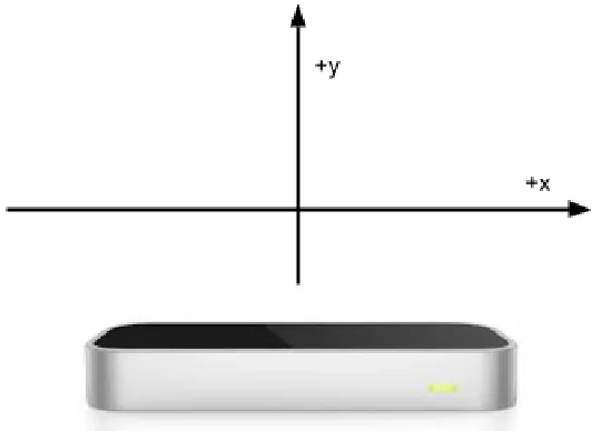
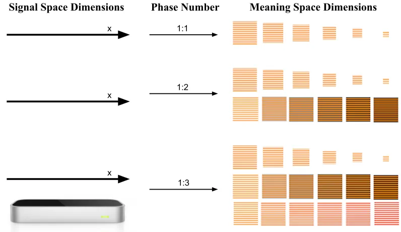
the hand within a horizontal dimension (x), vertical dimension (y) or both (Figure 1). Signals were generated
262
that either differed in pitch (on the x-axis), volume (on the y-axis), or both. Participants were told explicitly
263
which signal dimension(s) they were manipulating. When a signal could be altered along two perceptual
264
dimensions (i.e. pitch and volume), participants achieved this by moving one hand within a two-dimensional
265
space, i.e. moving a hand up or down would affect the volume, while a hand moving left or right would
266
manipulate the pitch. Participants could hear the signals they were producing. Participants were given clear
267
instructions on how to use the sensor and had time to get used to the mapping between their hand position
268
and sound.
269
Both the pitch and volume scales used were non-linear. Though our paradigm allows for any mapping
270
between the hand position and the acoustic signal, participant feedback in pilots indicated that people could
271
more intuitively manipulate non-linear scales. However, the output data has variables for both absolute hand
Figure 1. The signal dimensions available using theLeap Motion. In phases with a one-dimensional signal space, only either the x- or y-axis was available.
position within signal trajectories (represented as coordinates), and transformed pitch and volume values so
273
that we could explore whether participants were relying more on hand position or the acoustic signal.
274
Recording was interrupted when participants’ hands were not detectable, meaning that there were
275
no gaps in any of the recorded signals, even if participants tried to produce them. This was done to stop
276
participants creating gaps to separate structural elements in the signals, as this is not something typically used
277
to separate combinatorial elements in speech or sign. The data does not show much (if any) evidence that
278
participants tried to include gaps in the experimental rounds, which would be evident from sudden changes
279
in pitch in the signal.
280
The meaning space. The meaning space consisted of a set of squares that differed along continuous
281
dimensions. In phases where the meaning space only differed on one dimension, five black squares differed
282
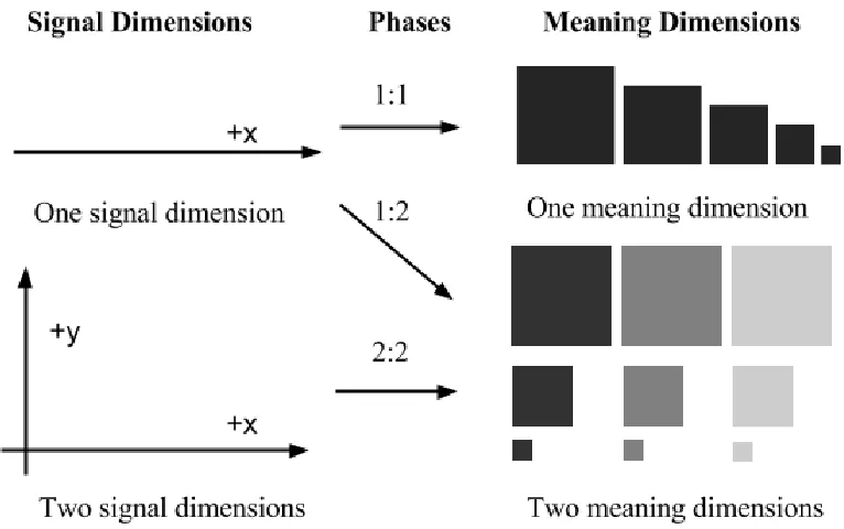
only in size. In phases where the meaning space differed on two dimensions, nine squares differed in both
283
size and in different shades of grey (Figure 2). Participants had to create distinct signals for each square.
284
Procedure. Participants were given instructions on how to generate signals using theLeap Motion.
285
They were given time to practice using theLeap Motionwhile the instruction screen was showing.
Partic-286
ipants had control of when to start the experiment, and so could practice for as long as they wanted. They
were instructed to sit back in the chair during the experiment, so that their upper body did not interfere with
288
theLeap Motion. Participants were also told that they would have to recognise the signals they produced, so
289
they knew they had to make signals distinct from one another.
290
There were three phases of the experiment: each phase consisted of a practice round and an
experi-291
mental round. There was no difference between practice rounds and experimental rounds, but only the data
292
from the experimental round was used in the analysis. Each practice and experimental round consisted of a
293
signal creation task and a signal recognition task.
294
Signal Creation Task. At the beginning of each signal creation task, participants saw the entire
295
meaning space. They then were presented with squares in a random order, one by one, and pressed an
on-296
screen button to begin and finish recording their signals. They had the opportunity to play back the signal they
297
had just created, and rerecord the signal if they were not happy. Participants created signals for all possible
298
squares in a phase.
299
Signal Recognition task. After each signal creation task, participants completed a signal
recog-300
nition task. All signals they had created were presented to them in random order one after the other. For
301
each signal, they were asked to identify its referent from an array of three randomly selected meanings (from
302
the repertoire of possible meanings - i.e. squares of different colours and shades of grey - within the
cur-303
rent phase) plus the correct referent, so four meanings in total. They were given immediate feedback about
304
whether they were correct, and if not, what the correct meaning had been. This task worked as a proxy for
305
the pressure to communicate each meaning unambiguously (expressivity), as participants knew that they had
306
to produce signals that they could then connect back to the meaning in this task, thus preventing them from
307
producing random signals, or just the same signal over and over again. Their performance in this task was
308
recorded.
309
When participants were incorrect, we measured the distance between the meaning they selected and
310
the correct meaning. The distance was calculated as the sum of differences along each dimension using a
311
measure similar to Hamming distance. Letmi jdefine a meaning with sizeiand shade jin a meaning space
312
where 0<i<Iand 0<j<J. The distance between two meaningsmi jandmi0j0 is then the following:
D(mi j,mi0j0) =i−i
0 +
j−j
0
(1)
For example, if the correct square has values 3 and 3 for size and shade respectively, and the chosen
314
square had vales 1 and 2 for size and shade respectively, the distance between these two squares would be 3.
315
Correct answers have a distance of 0.
316
Phase 1:1. All participants started with phase 1:1. In this phase, the meaning space consisted of five
317
black squares, each of different sizes (one meaning dimension). In this phase, the signal space also had only
318
one dimension, which was either pitch or volume. Which signal dimension the participants started with was
319
assigned at random. This phase was a matching phase, as there was a one to one mapping possible between
320
the meaning space and signal space (Figure 2).
321
Phase 1:2. In phase 1:2, participants created signals for a two-dimensional meaning space with the
322
squares differing in size and shade. The signal space had only one dimension. Participants used the same
323
one-dimensional signal space that they used in phase 1:1, so if they started the experiment only using pitch,
324
they only used pitch in this phase. This was the mismatch phase, as there were more meaning dimensions
325
than signal dimensions (Figure 2).
326
Phase 2:2. In phase 2:2, participants described the two-dimensional meaning space (differing in
327
size and shade), but with a two-dimensional signal space, where the signals differed in both pitch and volume
328
along the x and y dimensions respectively (Fig. 2). This phase was a matching phase also, as there was a one
329
to one mapping available between signal and meaning spaces.
330
Counterbalancing. Participants completed the phases in order 1:1, 1:2, 2:2 (where mismatch phase
331
interrupts matching phases) or 1:1, 2:2, 1:2 (where matching phases are consecutive). Order was
counter-332
balanced because participants’ behaviour may depend on what they have previously done in the experiment.
333
If people must solve the dimensionality mismatch before being presented with the two-dimensional signal
334
space, then they may continue using an already established strategy that only uses only one dimension, rather
335
than change their strategy to take advantage of both dimensions.
Figure 2. The phases used in the experiment. Phase 1:2 is the mismatch phase.
Post-experimental questionnaire. We administered a questionnaire with each participant after they
337
had completed the experiment. This questionnaire asked about the ease of the experiment, as well as about
338
the strategies that the participant adopted during each phase of the experiment. The questionnaire asked
339
explicitly whether they had a strategy and, if so, how the participant encoded each meaning dimension into
340
their signal.
341
Results
342
Signal Creation Task
343
The data collected from the signal creation task consisted of coordinate values designating hand
posi-344
tion at every time frame recorded, which is what the following statistics are based on. There were
approxi-345
mately 110 time frames per second. Signals were on average 3.36 seconds long. We first looked at the mean
346
of the coordinate values for each trajectory, and the duration of each signal. These simple measures give a
347
good starting point to assess whether participants were encoding the meaning space directly with the signal
348
space. If size or shade was directly encoded by pitch, volume or duration trough relative iconicity, then this
The first dimension a participant used was collapsed into one outcome variable in our analysis,
re-351
gardless of whether it was pitch or volume. All coordinates for signals using either pitch or volume were
352
normalised to have the same range. We also controlled for whether these coordinates were pitch or volume in
353
the mixed linear models below as a fixed effect, and also ran a separate analysis that showed that participants
354
performed just as well in the task when starting with either pitch or volume (reported in the signal recognition
355
results below). As explained above, meaning dimensions were coded to reflect the continuous way in which
356
they differed, i.e. the smallest square was coded as having the value of 1 for size, and the biggest square a
357
value of 5, with the lightest grey square given a value of 1 for shade, and the darkest had a value of 3. Using
358
these values, we could predict duration and mean coordinates from size and shade.
359
We ran a mixed linear model with size and shade as predictors, duration and mean coordinate value
360
as outcomes. Participant number was included as a random effect, and whether their starting dimension
361
was pitch or volume as a fixed effect. P-values were obtained by comparing with null models that did
362
not include the variable of interest. In the first phase, duration was predicted by the size of the squares
363
(χ2(1) =18.5,p<0.001), but the mean coordinate value was not. In the other 2 phases, the mean coordinate
364
of signals on the first dimension that a participant saw in phase 1:1 (either pitch or volume) was predicted most
365
strongly by shade. A mixed linear model, controlling for the same effects as above, showed this interaction
366
to be significant (χ2(1) =341.4,p<0.001). The duration of the signal was predicted most strongly by the
367
size of the square, with each step of size increasing the signal by 75.296 frames±7(std errors) (approx 0.7
368
seconds). The mixed linear model for this effect, controlling for the same fixed and random effects, was also
369
significant (χ2(1) =103.14, p<0.001). These effects demonstrate a propensity for encoding the meaning
370
space with the signal space using relative iconicity. Size and duration are easy to map on to one another,
371
and it makes sense that participants are more likely to encode the remaining meaning dimension (shade) with
372
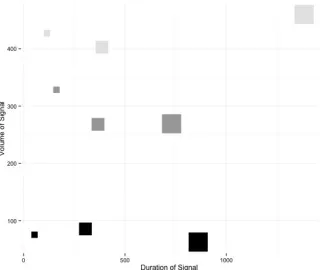
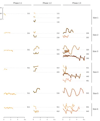
the signal dimension they were first exposed to. Figure 3 shows the output of one participant who mapped
373
the signal space onto the meaning space in a very straightforward one to one mapping, with size encoded
374
with duration and shade encoded with volume. This is an example of a topology-preserving mapping (a
homeomorphism).
[image:17.612.148.468.155.425.2]376
Figure 3. The mean trajectory coordinates (in mm) along the axis manipulating volume (where lower values refer to louder sounds) plotted against duration (number of data frames, roughly 1/110 of a second). Size and shade are represented by the size and shade of the squares in the graph. Within the phase with the two-dimensional meaning space with a two-dimensional signal space, this participant used signal duration to encode size, and signal volume to encode shade.
We also looked at standard deviation in signals to give us a good idea of the amount of movement
377
in a signal. Signal trajectories produced in the phase where there was a mismatch (1:2) had higher standard
378
deviations (M= 48.2mm) than signals produced in phases where the signal and meaning spaces matched in
379
dimensionality (M= 33.4mm), indicating more movement in mismatch phases. Using a linear mixed effects
380
analysis with standard deviation as the outcome variable and whether phases were matching or mismatching
381
as the predictor, and controlling for participant number as a random effect, and whether they started with
382
pitch or volume as a fixed effect, we found a significant effect (χ2(1) =4.5,p<0.05).
We also quantified signal structure by measuring the predictability of signal trajectories given other
385
signals in a participantâ ˘A ´Zs repertoire. If each signal trajectory in a participant’s repertoire is predictable
386
from the other signals, this gives an indication of systematic and consistent strategies being used within the
387
repertoire.
388
We created a measure for predictability of each signal trajectory, derived from a participant’s entire
389
repertoire. The procedure is as follows:
390
1. Use the k-means algorithm to compute a set of clustersSof hand coordinates using the whole repertoire,
391
which reduce the continuous-valued trajectories to discrete ones (k=150).
392
2. Calculate the bigram probability distributionPfor each symbolxi∈S.
393
3. Use the bigram probabilities to calculate the negative log probability of each trajectory using Equation
394
2 below.
395
The choice of kwas set quite high at 150 to ensure the quantisation was sufficiently fine-grained.
396
This ensured that the high variation in our data set is well-represented in the prediction scores to avoid
397
overestimating similarity. In the literature, such high values for this parameter are used for modelling
high-398
dimensional speech data, which we used as an upper bound (e.g. Räsänen, Laine, & Altosaar, 2009).
399
LettingSbe the set of 150 clusters obtained in step 1, andT be a trajectory that consists ofmsymbols
400
x0,x1,x2, ...,xmwherexi∈S, the formal description of step 3 is the following:
401
P(T) =−logP(x0)− m
∑
a=1
logP(xa|xa−1) (2)
With the predictability value for each trajectory, we used a linear mixed effects model to compare the
402
predictability of signals in the matching and mismatching phases. Controlling for duration and participant
403
number as random effects, and size and shade of square as fixed effects, we found that whether signals
were produced in matched or mismatched phases predicted how predictable a trajectory was (χ2(1) =3.9,
405
p<0.05). Signals produced in the matching phases had higher predictability.
406
Signal Recognition Task
407
Overall, participants were good at recognising their own signals, identifying a mean of 66% of signals
408
correctly, where 25% was expected if participants performed at chance level. Using a linear regression model,
409
we found that participants improved by around 10% with each phase of the experiment (F(1,76) =9.96,
410
p<0.01).
411
There was no significant difference between the recognition rates of participants who started with
412
either volume or pitch (t(21.9) =−0.46, p=0.65), suggesting that there was no difference in difficulty
413
between the signal dimensions. We also used a linear regression model to test if musical proficiency predicted
414
performance in the signal recognition task, and found that it did not (F(1,23) =0.03,p=0.86).
415
If signals rely on relative iconicity, then similar signals will be used for similar meanings, causing
416
more potential confusion between signals for similar squares. This confusability may cause participants to be
417
worse at the signal recognition task when relative iconicity is more prevalent. We tested whether participants
418
were indeed worse at the recognition task in the condition where we predicted relative iconicity (in the
419
matching phases). In line with this hypothesis, we found that participants were worse at recognising their
420
signals within matching phases (1:1, 2:2) (M = 61.3% correct,SD24%), than in mismatching phases (1:2)
421
(M= 69.6%,SD= 21%). However, this result was not significant (t(53.3) =−1.5,p=0.13), and may be an
422
artefact of the experiment getting more difficult as it progressed.
423
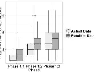
We also calculated the distances between incorrect answers and target answers, as discussed in our
424
methods (Signal Recognition Task section). To compare these values to a baseline, we also calculated the
425
distance between the target answer and a randomly chosen incorrect answer. Comparing the actual data with
426
the random data using a mixed effect linear model, and controlling for participant number as a random effect,
427
and stimulus number as a fixed effect, we found that with incorrect choices produced in the matching phases
428
(1:1, 2:2), participants were closer to the correct square (M= 2.6 steps away,SD= 1.4) than if they had chosen
there was no difference between actual incorrect choices and random incorrect choices (both around 3.6 steps
431
away,χ2(1) =0.01,p=0.9). Further, we found that the distance from the correct answer was much higher
432
in the mismatching phases (M= 3.6 steps away,SD= 1.5), than in the matching phases (M= 2.6 steps away,
433
SD= 1.4), indicating that participants were relying more on relative iconicity in the matching phases, because
434
their mistakes were predicable, assuming a transparent mapping between the signal space and the meaning
435
space. We tested this using a mixed effect linear model, and controlling for the same variables found the
436
effect was significant (χ2(1) =5.3,p<0.05).
437
Post-experimental questionnaire
438
Nearly all participants reported strategies and they were mostly the same strategies. These strategies
439
included using pitch, volume or duration directly to encode size or shade. For example, many participants
440
used high pitches or short durations for small squares and low pitches or long durations for big squares.
441
Participants also reported that involved different movement types, frequencies and speeds.
442
As we predicted in the section on counterbalancing, participants who saw phase 1:2 before phase 2:2,
443
were more likely to use the same signal strategy throughout, than to change the strategy to take advantage
444
of both dimensions. 84% (SD= 37%) of strategies used for a particular meaning dimension were consistent
445
throughout phases 1:2 and 2:2 by participants who saw 1:2 first. Only 54% (SD = 50%) of strategies by
446
those who saw 2:2 first were consistent. Consistency rates between different phase orders were significantly
447
different (χ2(1) =8.7,p<0.01).
448
Whether a participant self-reported as having a strategy or not influenced their performance in the
449
signal recognition task. Participants were significantly more likely to perform better at recognising their own
450
signals in a given phase, if they reported having a strategy (M=70% correct,SD= 20%), than if they didn’t
451
(M=40% correct,SD= 16%) (t(26.6) =−6,p>0.001).
452
Hidden Markov Models
Models. While our predictability values outlined in the previous sections are useful to characterise
454
internal similarities in a repertoire, the clustering algorithm they are based on ignores temporal dependencies.
455
To infer the structure of the signal repertoires including the temporal dependencies, we used Hidden Markov
456
Models, or HMMs. An HMM consists of a set ofstatesof which only one can beactiveat a time. The active
457
state produces observableemissions(such as short stretches of time) drawn from a state-specific distribution,
458
and the next active state depends only on the currently active state. In the models we derive from our
experi-459
mental data, states are analogous to phonemes (or similar to building blocks), and the emission distributions
460
to determine how they are realised phonetically. By training HMMs on the signal repertoires, we can estimate
461
the most likely vocabulary of states across a repertoire, i.e. the most likely “phonological” alphabet. Note
462
that this model does not explicitly include meanings, since our purpose is to model the structure of the signal
463
repertoire.
464
HMMs are very common in natural language processing applications, such as part-of-speech tagging
465
and speech recognition (Baker et al., 2009). A common use for HMMs in the field is modelling phonemes,
466
where typically three states represent three phoneme positions, and their emissions are very short segments
467
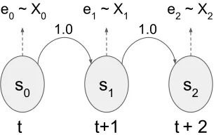
of speech making up the observed signal (seeFigure 4).
468
s
0s
1s
2e0 ~ X0
t
t+1
t
+ 2
1.0 1.0
[image:21.612.230.384.462.558.2]e1 ~ X1 e2 ~ X2
Figure 4. A simple, three state, left-to-right HMM emitting the observation sequencee0e1e2through the state
sequences0s1s2. Each observationeiis a random sample from the emitting state’s emission distributionXi
wherei∈ {0,1,2}. Transitions are annotated with their probabilities. Note how the only non-deterministic part of the system is the emissions in this type of HMM.
HMMs are typically used with a fixed transition matrix and a fixed number of states. Each phoneme is
469
modelled as a “left-to-right” HMM. These models have exactly one possible starting state, and all transitions
470
are deterministic. Further, applications typically assume the number of states is already known and only
whose structure is familiar (such as human speech), it is not a very useful method of discovering and/or
473
characterising structure in signals where the properties of the signalling system are unknown. Most of the
474
structural variation available is ruled out by the fixed architecture of the HMM. Furthermore, contrary to
475
common practice, we are interested in modelling the properties of the whole signal repertoire rather than
476
individual signals.
477
Since we use HMM as a model of the speaker, the estimated properties of the model should be able
478
to predict the participant’s performance, such as their score in the recognition task for that phase. In
partic-479
ular, we are interested in whether the number of states in the HMM can predict the recognition score of a
480
participant. Since the states are analogues for the phonemic inventory, we predict participants with bigger
481
inventories will have worse recall. Such predictive power would indicate the model successfully captures
482
aspects of participant behaviour during the experiments.
483
We propose that fewer building blocks across a repertoire indicates combinatorial strategies in
compar-484
ison to strategies of relative iconicity. The efficiency that combinatorial structure brings is due to its capability
485
to encode multiple meanings with combinations of a limited number of fundamental building blocks (or states
486
in the HMMs). We expect combinatorial strategies (represented by a smaller numbers of states) to be more
487
efficient in communicating meanings, because they overcome the problem of crowding in the signal space
488
resulting in less confusion between signals. On the other hand, a system with relative iconicity, which would
489
have to maintain a systematic relationship between the meanings and forms, would result in many states
490
within a crowded system. With a combinatorial system, encoding a newly encountered meaning dimension
491
does not require the invention of a new signal dimension to provide a range of signals to encode variations on
492
the meaning dimension, which is what would happen with relative iconicity. We predict that the signals from
493
phases where the number of meaning dimensions is greater than the number of signal dimensions will have
494
combinatorial structure, and this will manifest itself in HMMs trained on those signals havingfewerstates
495
than signals from matching phases.
496
We calculate the structure as well as the transitions of HMMs, with only an upper boundary on the
number of states and no constraints on transitions. We use HMMs with continuous multivariate (Gaussian)
498
emissions and the standard Baum-Welch algorithm for unsupervised training. We trained a separate HMM
499
on the set of signals generated by each participant at each phase of the experiment. This way, we ensured that
500
all signals that went into training a particular HMM had been created to label the same meaning space.
501
Because the mapping between hand position and the tones generated is non-linear, it makes a
differ-502
ence to the HMM which representation we use to train it. Which one works best depends on how participants
503
memorise signals. There is no way of knowinga prioriwhether the participants will memorise (and when
504
playing as the hearer, reverse-engineer) the hand movements themselves, or the tones produced by these
505
movements. So, in addition to the raw data that assumes the states emit hand coordinates, we trained the
506
models on two transformed data sets that assume the emissions are tonal amplitude and frequency values.
507
These two additional sets varied in their frequency units, one using the Mel scale and the other Hertz. The
508
full training procedure used for each projection is presented inAlgorithm 1inAppendix A.
509
A series of linear mixed effects regressions were run to see what aspects of the HMMs are most useful
510
in predicting the signal recognition scores. The dependent variable and covariates we have considered are
511
the number of states of the model, while the predictors were phase, phase presentation order, and whether
512
the phase is matching or mismatching. The random effects were whether volume or pitch was the first signal
513
dimension introduced, and the participant number. Likelihood ratio tests were used to justify every additional
514
component to the regression equation, corrected for the number of comparisons. The details of the regression
515
and estimated coefficients are inAppendix B. Phases are coded as p∈ {1 : 1,1 : 2,2 : 2}, independent of
516
their presentation order (seeCounterbalancingin the Methods section for explanation about order of the
517
phases). Order of presentation is taken into account in the analysis, and is coded as "consecutive" (when the
518
matching phases appear one after the other) or "interrupted" (when the mismatching phase appears between
519
the matching phases). The matching phases arep∈ {1 : 1,2 : 2}, and the mismatching phase is 1 : 2.
520
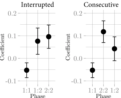
Experiment 1 HMM Results and Discussion. The interaction of number of states, phase order and
521
mismatch was the best predictor for participant score in each phase (R2=0.616). The signal representation
522
most successful in predicting the recognition score was the Mel frequency and the amplitude in linear scale.
Some combinations of the interacting components were logically excluded; for instance, the 1:1 phase
525
can only take place in the first position, so there is no coefficient for the interaction between the 1:1 phase
526
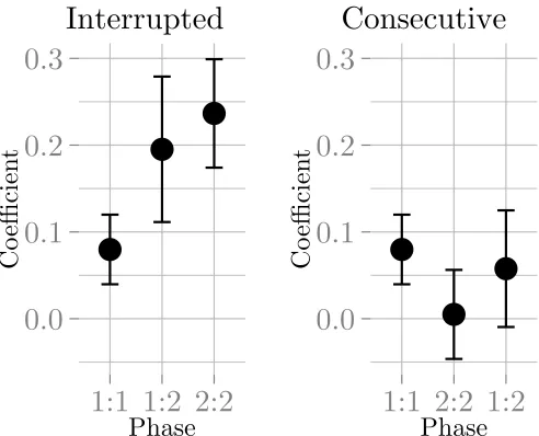
and phase orders other than 1. SeeFigure 5for the regression coefficients.
527
0.0
0.1
0.2
0.3
1:1 1:2 2:2
Phase
Co
efficien
t
Interrupted
0.0
0.1
0.2
0.3
1:1 2:2 1:2
Phase
Co
efficien
t
[image:24.612.182.428.199.398.2]Consecutive
Figure 5. Fixed effects from Experiment 1, for both orders of presentation of phases. Each coefficient represents the estimated number of extra states a phase requires in that condition. Phases 1:1 and 2:2 are matching phaes. Phase 1:2 is mismatching.
The coefficients associated with predictors reveal a somewhat complex picture (Figure 5). Considering
528
that the coefficients indicate the increase or decrease in the number of states required in each condition to
529
achieve the same recognition score compared to the baseline, the coefficients suggest:
530
• There is a clear distinction between different orderings 1:1, 1:2, 2:2 (interrupted) and 1:1, 2:2, 1:2
531
(consecutive). The required number of states is minimised for the consecutive ordering
532
• For either ordering, the need for any more or fewer states when moving from the second phase to the
533
third phase is insignificant.
534
• Whether the second phase requires more or fewer states than the first depends on whether the second
535
is a match or a mismatch.
Our results cannot confirm the prediction that mismatching phases would require fewer HMM states.
537
It seems that our prediction only holds for the interrupted ordering where there is a monotonic (but not
538
necessarily significant) increase in the number of states required.
539
If the matching phases are consecutive (1:1, 2:2, 1:2), this seems to help all future phases to reduce
540
the number of required states compared to the first phase (although only the difference between the first and
541
the third phases is significant). However, if the matching phases are interrupted by the mismatching phase
542
(1:1, 1:2, 2:2), every phase requires more states than the one it follows (both second and third phases require
543
significantly more states than the first). This different behaviour based on ordering is visible in the how the
544
coefficients for phases 1:2 and 2:2 have markedly different values in the left and right panels of figure 5.
545
Strikingly, the phase that required the least number of states across all data seems to be phase 2:2 presented
546
as the second phase. This is despite phase 2:2 mapping on to a meaning space twice as large as 1:1.
547
Order of presentation causing participants to break strategy has an effect beyond whether or not a
548
phase is mismatching. For instance, in the ordering 1:1, 1:2, 2:2, the participant could simply ignore the
549
additional dimension on the final phase to perform at least as well as the second phase, yet there is an
550
(insignificant) increase in the coefficient in the 2:2 phase. Interestingly, the opposite trend can be seen in
551
the other ordering, where changing over to a mismatching phase results in an (insignificant) increase in the
552
number of states required.
553
Experiment 2
554
Experiment 1 provided important evidence of the effects of matching and mismatching signal and
555
meaning space topologies. When there is a one to one mapping between signal and meaning spaces,
par-556
ticipants tend to take advantage of it. Indeed, even in our conditions designed to produce a dimensionality
557
mismatch, participants used duration as another signal dimension. Despite this, we were still able to find
558
significant effects of the matching phases compared to the mismatching phases on the amount of movement
559
in signals, the consistency of iconic strategies and how predictable recognition mistakes were.
560
Experiment 2 was a very similar signal creation experiment. It tested the same hypothesis as
1) Duration was used as a dimension by some participants, meaning there wasn’t really a “mismatch"
563
even with the 1:2 phase.
564
2) Participants created signals for a very small meaning set in Experiment 1 (5 or 9 meanings
depend-565
ing on the phase), which was seen in its entirety before the experiment. This made it easier for participants to
566
create a completely holistic signal set without the need for structure. Only one participant treated meanings
567
holistically in Experiment 1 (using frequencies of pitch contours to differentiate meanings). However, we
568
feel that this is still a flaw in the experimental design, as this strategy would soon become maladaptive as
569
meaning numbers rise. In the real world, continuous meaning dimensions are much more nuanced than only
570
having 3 or 5 gradations.
571
To counter these problems, two alterations have been made in Experiment 2:
572
1) Phase 1:2 in Experiment 2 has been dubbed a “match" phase, and a new phase 1:3 has been instated
573
to be sure there is a dimensionality mismatch.
574
2) Participants do not create signals for every possible meaning, but a subset of them. This is explained
575
further in theMeaningssection below.
576
Methods
577
Participants. Participants were recruited at the VUB in Brussels. 25 participants took part in the
578
experiment; 8 male and 17 female. Participants had an average age of 21 (SD= 3.2). As in Experiment 1,
579
we asked participants to list the languages they speak, with level of fluency, and to self-report their musical
580
proficiency (on a scale of 1-5).
581
Signals. As in the first experiment, there was a continuous signal space built using theLeap Motion
582
sensor to convert hand motion into sounds. However, in this experiment, signals could only be manipulated
583
in pitch. Participants manipulated the pitch in the same way as in Experiment 1, along the horizontal axis.
584
There was an exponential relationship between hand position co-ordinates and signal frequency. The vertical
585
axis was not used at all in this experiment, meaning that, including duration, the number of signal dimensions
could not be more than 2. However, participants were not explicitly told to use duration in order to make
587
the results from Experiment 1 more comparable with Experiment 2. Again, participants were given clear
588
instructions on how to use the sensor, and were given a practice period to get used to the mapping between
589
the position of their hand and the audio feedback before the experiment started.
590
Meanings. The meaning space again consisted of a set of squares, but in this experiment they
dif-591
fered along three continuous dimensions: size, shade of orange, and shade of grey. Squares differed along
592
different numbers of dimensions in each phase (Figure 6). In contrast to the first experiment, participants
593
only saw a subset of the possible meanings. Each dimension was divided into 6 gradations, meaning that the
594
meaning space grew exponentially with the number of dimensions (see description of phases below). Having
595
6 gradations of difference on meaning-space dimensions meant the meaning space is big enough to have
596
make productive systems useful, but coarsely grained enough to not make the discrimination task impossible.
597
Further to the reasons given above, this aspect of the experimental design made an incentive for participants
598
to create productive systems that extend to meanings they have not seen. The subset the meanings participants
599
saw were randomly selected, but participants were explicitly told about all of the possible dimensions. This
600
pressure to make productive systems because one has only seen a subset of a bigger meaning space has been
601
demonstrated in experiments such as Kirby et al. (2008) and Kirby, Tamariz, Cornish, and Smith (2015).
602
Two of the meaning dimensions in this experiment were “shade of grey" and “shade of orange". In
603
pilot studies, we originally had the squares differ in shade of orange (which we controlled using the RGB
604
ratio of green to red) and the brightness value. However, this made the squares at the darker and redder end
605
of the scale very difficult for participants to tell apart, as they all appeared the same dark brown colour. To
606
solve this, we used striped squares with alternating grey and orange stripes (see figure 6). This gives the same
607
effect of squares differing in shade of orange and brightness, but squares at both ends of the spectrum can be
608
distinguished just as easily.
609
Procedure. The procedure in Experiment 2 was nearly the same as Experiment 1. There were still
610
3 phases, each with a practice round and an experimental round, which were both the same. Each round has
611
a signal creation task and a signal recognition task. However, the phases were slightly different.
1:1
1:2
1:3 x
x
[image:28.612.107.505.98.328.2]x
Figure 6. The signal and meaning dimensions used in experiment 2 in each of the 3 phases.
Phases. All participants had phases presented in the same order: 1:1, 1:2, 1:3. The "1" here refers
613
to 1 signal dimension (pitch), in order to make these phase labels consistent with the phases in Experiment 1.
614
However, since we have learnt to expect participants to use duration as a signal dimension, it is important to
615
remember that the meaning dimensions only outnumber the signal dimensions in a meaningful way in phase
616
1:3.
617
Phase 1:1. In phase 1:1, there were 6 squares that differed in 6 gradations of size. All 6 squares
618
were presented in a random order.
619
Phase 1:2. In phase 1:2, there were 36 possible meanings. Meanings differed along two dimensions,
620
6 gradations of size and 6 shades of grey stripes (See Figure 6.) 12 meanings were chosen at random from
621
this set of 36. Participants were then presented with them in a random order. Participants were explicitly told
622
about the introduction of the new meaning dimension at the beginning of the phase.
623
Phase 1:3. In phase 1:3, participants were presented with 12 squares in a random order that differed
624
along three dimensions, 6 gradations of size, 6 shades of grey stripes and 6 shades of orange stripes (See
625
Figure 6.) This made a possible number of 216 squares, which were chosen from at random. This does mean
that some participants saw more “evidence" of some dimensions than others in the subset of squares that
627
they saw. However, as with phase 1:2, all participants were explicitly told about the introduction of the third
628
meaning dimension at the beginning of the phase.
629
Signal Recognition task. As in the first experiment, participants completed a signal recognition
630
task. They heard a signal they had created, and were asked to identify its referent from an array of three
631
randomly selected squares from the set of possible squares in the current phase, plus the correct referent, so
632
four squares in total. They were given immediate feedback about whether they were correct, and if not, what
633
the correct square had been. Their performance in this task was recorded for use in the analysis. The distance
634
in the meaning space they were from the correct answer was also recorded in the same way that it was in
635
Experiment 1.
636
Post-experimental questionnaire. The questionnaire asked about the strategies that the participant
637
adopted during each phase of the experiment. As in the first experiment, the questionnaire was free-form.
638
Participants were also asked to name the 6 shades of orange used in the experiment, in order to see if they
639
did indeed label them all "orange", and to see if and how they categorised the colours affected their signals.
640
The shades used in the experiment had been designed to all be perceived as orange. Only 17 participants
641
completed this later part of the questionnaire because of experimenter error.
642
Results
643
Signal Creation Task
644
Descriptive Statistics
645
In this experiment, signals were on average 2.3 seconds (approx. 252 frames long). The average
646
duration of signals rose by about 20 frames each phase (χ2(1) =7.9,p<0.005).
647
As in Experiment 1, meaning dimensions were coded to reflect the continuous way they differed, i.e.
648
the smallest square was coded as having the value of 1 for size, and the biggest square a value of 6, while
649
the lightest grey/orange stripes were given a value of 1 for shade/colour, and the darkest had a value of 6.
650
Again, across all phases, the size of square was the best predictor for the duration of the signal (χ2(1) =63.3,
the largest squares having a mean duration of 2.7 seconds (SD= 1.9s). However, in this experiment size was
653
also the best predictor for the mean pitch of the signals (χ2(1) =15.7, p<0.001). The smallest squares had
654
a mean pitch of 403Hz, and the largest squares had a mean pitch of 333Hz. Again, we take this as evidence
655
for the use of relative iconicity.
656
We again looked at the standard deviations of individual signal trajectories to see if the degree of
657
mismatch in the signals affected the amount of movement in the signals. There was no significant difference