Biologically inspired 3D face recognition from surface normals

Biologically inspired 3D face recognition from

surface normals

Mark F. Hansen, Gary A. Atkinson

Machine Vision Laboratory, University of the West of England,

Bristol. BS16 1QY.

Abstract

A major consideration in state-of-the-art face recognition systems is the amount of data that is required to represent a face. Even a small (64×64) photograph of a face has 212_{dimensions in which a face may sit.}

When large (>1MB) photographs of faces are used, this represents a very large (and practically intractable) space and ways of reducing dimension-ality without losing discriminatory information are needed for storing data for recognition. The eigenface technique, which is based upon Principal Components Analysis (PCA), is a well established dimension reduction method in face recognition research but does not have any biological ba-sis. Humans excel at familiar face recognition and this paper attempts to show that modelling a biologically plausible process is a valid alternative approach to using eigenfaces for dimension reduction. Using a biologically inspired method to extract the certain facial discriminatory information which mirrors some of the idiosyncrasies of the human visual system, we show that recognition rates remain high despite 90% of the raw data being discarded.

1

Introduction

Face recognition has been an area of intense research for over forty years and, although significant progress has been made, a number of major challenges remain. Much of the research focuses on face recognition using 2D images which has highlighted some universal problems that affect recognition accuracy. Two of these problems, pose and illumination variance, can be compensated for using 3D models rather than 2D photographs. Because of this, and the increased availability of 3D capture devices, 3D face recognition has become an active research area over the past decade.

processes underlying human face recognition are still poorly understood and 2) good results are achieved using classical pattern recognition approaches.

The motivation for this work therefore comes from attempting to improve aspects of automatic face recognition by incorporating features of the HVS. In particular we look at dimension reduction and present a method based upon the idea of caricaturing that was theorised by Unnikrishnan [2]. By only using facial data which falls outside the 5th_{and 95}th _{percentiles for a given face database}

(i.e. 90% is discarded) we show that recognition rates only show a proportionally small decrease thus lending support to Unnikrishnan’s hypothesis.

1.1

Related work

Early research into automatic face recognition focused on describing a face in terms of absolute or ratios of distances between features [3, 4, 5]. Information theory inspired a new statistical approach termed eigenfaces by which Principal Components Analysis (PCA) is used to describe a face in terms of a linear com-bination of coefficients [6]. Recognition is is then performed using the smallest Euclidean distance between the coefficients of a probe image and the mean co-efficients for each identity within the gallery. This approach has the advantage of not needing to mark and measure fiducial features on the faces as was neces-sary with the earlier approaches. The Fisherface technique [7] incorporates class information (in this case the identities of the photographs) in order to find a better dimensional representation which maximises the clustering of the classes, making discrimination easier. Both eigenfaces and Fisherfaces are commonly used in state-of-the-art research as they represent acknowledged benchmarks, with Fisherfaces providing better recognition performance as long as there are sufficient training examples [8]. For this reason, the Fisherfaces technique is adopted for use in this paper.

A different and biologically motivated approach comes from using Gabor filters [1, 9, 10]. The Gabor filter [11] is fundamentally a sine wave windowed by a Gaussian. By varying the orientation and frequency of these waves, filter banks which mimic functionality of an area in the primary visual cortex (area V1) are created [12, 13]. In the approach used by Wiskott et al. [10], it is not necessary to mark out fiducial features, as an elastic bunch graph map (EBGM) finds the features most similar to those in its database automatically. Testament to the benefits of using biologically inspired Gabor filters comes from the FERET [14] evaluation and FVC2004 [15] face recognition tests, in which the top performing algorithms used Gabor filters for feature extraction.

The main drawback of implementing Gabor filters is that they are computa-tionally intensive. More efficient alternatives are Local Binary Patterns (LBP) which approximate the Gabor function. This approach is most commonly as-sociated with face detection e.g. [16] but it has also been used successfully for face [17] and even expression recognition [18].

features which are directly involved with human face recognition can be found in [19] including caricaturing. Caricaturing can be defined as the exaggeration of features away from the average e.g. if someone has a larger than average nose, the caricature would exaggerate the nose to make it even larger. Caricaturing essentially enhances those facial features that are unusual or deviate sufficiently from the norm. It has been shown that humans are better able to recognise a caricature than they are the veridical image [20, 21]. This finding is interesting as caricaturing is simply distorting or adding noise to an image, but this noise aids human recognition and this, in turn, provides insights into the storage or retrieval mechanism used by the human brain.

Unnikrishnan [2] conceptualises an approach similar to face caricatures, whereby only those features which deviate from the norm by more than a thresh-old are used to uniquely describe face. Unnikrishnan suggests using those met-rics whose deviations lie below the 5th_{percentile and above the 95}th_percentile,

thereby discarding 90% of the data. Apart from dimension reduction, an in-teresting feature of this approach is that because it is norm-based, faces from under-represented groups (in our case ethnicity and gender) will possess fea-tures not present in the average population. These feafea-tures are distinguishing to that group leading to a clustering of minority groups making discrimination for difficult. This is analagous to a well documented feature in human face recognition known as theown-race effect [22] by which discrimination of faces from races other than the subject’s own is diminished. No empirical support for Unnikrishnan’s hypothesis is given in [2], so the aim of this paper is to test the presented theory.

Most face recognition experiments in the research literature are carried out using 2D photographs, but it has been shown that 3D models lead to improved recognition rates because illumination and pose can be compensated for [23], although this finding is not always replicated [24]. The database used for the experiments in this paper consists of surface normal data captured using the PhotoFace device (Fig. 1). PhotoFace is a 3D photometric stereo capture system which was placed in a workplace corridor for six months and left to capture unconstrained images of employees walking through the device (for more details, the interested reader is referred to [25]). Photometric stereo is a technique of illuminating an object from multiple directions and using the known positions of illuminants and pixel intensity to estimate surface orientation [26]. Surface normal data is particularly well suited to face recognition as shown by G¨okberk in his meta-analysis [27] on the effect of different data representations for face recognition. He concluded that “. . . surface normals are better descriptors than the 3D coordinates of the facial points.”.

Figure 1: The PhotoFace capture device. The insets show a flashgun light source and the ultrasound trigger, which detects the presence of a person using the device.

we term theown-sex effect by which we might expect worse recognition on the gender which is under-represented. (NB There is no evidence for the own-sex effect in human recognition, probably because exposure to one sex over another to the same levels as to generate the own-race effect is not feasible).

1.2

Contributions

The contributions of this paper are four-fold:

• We show that discarding 90% of facial data by only keeping the outlying 10% just leads to a 24% drop in recognition performance on 3D surface normal data.

• The drop in performance using 2D data, on the other hand, is much greater (a drop of 43%).

• This provides empirical support for Unnikrishnan’s hypothesis concerning the important discriminatory properties of outliers.

• We show that 3D surface normal data gives better recognition perfor-mance than 2D photographs on a database of images captured in an un-constrained “real world” environment.

2

Data and Methodology

The data used for our experiments consists of 61 subjects with at least six sessions each (that is six sets of photometric stereo images per subject). All images were taken in a frontal pose with neutral expression. The maximum number of sessions per subject is 70, the mean number of sessions per subject is 16 with a mode of 7. Of the 61 subjects, only two are female, and only one is not caucasian - these are the subjects whose sessions are used for exploring the own-race/sex effect. There are a total of 1000 sessions. Four images are captured per session with different illuminants in ≈20ms. This effectively freezes the subject’s motion. For these experiments, visible light flashguns are used (colour temperature≈5600K). A standard photometric stereo technique [28, Section 5.4] is then used to estimate the surface normals at each pixel. Although not used in this paper, the normals can be integrated to form a surface via, for example, the well known Frankot-Chellappa method [29]. An example set of images can be seen in Fig. 2.

The centre of the eyes and nasion are manually labelled on each image. The images are then scaled and aligned to one another. Fig. 3 shows how the face region is cropped based around the distance between the centres of the eyes. This results in a close crop around the eyes nose and mouth, and excludes areas such as the chin and forehead which can frequently be covered with hair and are therefore unreliable features for recognition. Due to memory limitations the images are then scaled down to 80×80px.

In order to remove any artefacts which are caused by the flashguns having different brightness, the greyscale intensity of the images is normalised. This is achieved by making the mean of each image the same as the mean of all session images. Other normalisation techniques such as histogram equalisation, contrast limited adaptive histogram equalisation and increasing the range of intensity values to a maximum 0-255 were investigated in terms of their effect on recognition performance, but none offered any improvement.

The images that we use for 2D recognition are generated by taking the mean of each pixel of the four differently lit images. This reduces any confounding influence of illumination variance that may be present if only one lighting con-dition were used e.g. extreme lighting and cast shadows. Each mean image is reshaped into a vector and these vectors are added into a matrix such that columns represent sessions and rows represent greyscale intensities at a partic-ular pixel. As each mean image is 80×80px, the dimension of the matrix used for percentile calculation and subsequent recognition is 6400×1000.

Figure 2: Four differently illuminated images, the needle map of surface normals and the integrated surface

ycomponents of each session are reshaped and then concatenated into a single vector. In the same way as for the 2D mean images, these vectors are added into a matrix such that columns represent sessions and rows representxandy

components at a particular pixel. As there are 80×80 values for both thexand

ycomponent, each session is therefore represented by a vector 6400×2 = 12800 in length. The dimensions of the matrix are therefore 12800×1000.

In order to work out which data in each image falls in the outlying 10% of the data, we first need to calculate the thresholds for each pixel which represent the 5th _{and 95}th_{percentile values. This is a norm-based approach, and we are}

interested in the norm across the whole dataset for each pixel rather than the norm for each image. For the 2D photographs, percentile values are calculated for the greyscale intensity value for each pixel. There are 1000 sessions, so there are 1000 values for each pixel from which we calculate the 5th_{and 95}th_percentile

values. Once reshaped into the original dimensions, this results in two 80×80 matrices (one for the 5thand one for 95thpercentile), examples of which can be seen in Fig. 4. In the same way, for 3D surface normal data, percentile values are calculated forxandysurface normal component values for each pixel. Once these thresholds have been calculated, all pixels which have a value between the 5th_{and 95}th _{percentile are discarded, leaving only the 10% outlying data.}

The method used to test recognition accuracy is the leave-one-out paradigm. This dictates that every session is used as a probe against a gallery of all other sessions once. There are therefore 1000 classifications per condition of which the percentage correctly identified is shown.

Figure 3: Cropping the face images based on the inter-eye distance. The distance between the eye centres is denoted byd.

20 40 60 80 100 120 140

Base rate Outliers

2D photographs 91.2 30.2 3D surface normals 97.5 73.5

Table 1: Recognition rates (%) on 2D photographs and 3D surface normal data. The base rate column shows recognition rates for the raw data, and the outliers column shows recognition rates on the outlying 10% of data (data whose deviation lies below the 5thpercentile and above the 95thpercentile).

3

Results

Example data for two subjects can be seen in Fig. 5. 2D examples are shown in the eight images on the left, and 3D examples are shown on the right. The 3D examples only showy-component data to simplify visualisation – it should be noted that the experiments are also performed on thex-components. Each row represents data for one subject. The first two images on each row of the groups show examples of aligned and cropped greyscale intensity images (2D photographs) and rawy-component surface normals. The next two images show the corresponding outlying data of the first two images (i.e. those pixels with a value whose deviation lies below the 5th or above the 95thpercentile). There is visibly more consistency between the outlying 3D data than the 2D data, especially for the first subject.

Table 1 shows the baseline recognition rates for 2D and 3D data, as well as the rates using only the most outlying 10% of data. The table can be summarised as follows:

1. 3D surface normal data gives better recognition rates than 2D photographs (97.5% vs 91.2%)

2. Far better recognition is seen on the 3D outlying data than the 2D outlying data (73.5% vs 30.2%).

3. The decrease in performance when only the outlying 10% of data is used is only 24% on the 3D data which is disproportional to the 90% of data which has been discarded.

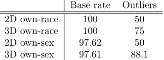
Table 2 is designed to investigate the own-race and own-sex effect. It is clear from the table however, that neither the own-race nor the own-sex effect are being exhibited as the performance drop of the outlying data is less than that across the whole group (as seen in Table 1). Caution should be exercised in any interpretation of these results as the number of sessions available for ethnic minority/female subjects is very small (one subjects with 16 sessions and two subjects with 42 sessions respectively). These results are discussed further in Section 4.

Base rate Outliers

2D own-race 100 50 3D own-race 100 75 2D own-sex 97.62 50 3D own-sex 97.61 88.1

Table 2: Recognition rates (%) for subjects using a single race/sex subset of the data.

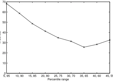
is generally contained in the outlying data than the rest of the data. It may be that there are other bands of percentiles which provide better recognition. This was investigated by measuring the recognition rate using different bands of percentiles e.g. [10-15, 90-95], [15-20, 85-90] etc. which account for 10% of the data. Fig. 6 shows a plot of the recognition rate against these bands and provides support for Unnikrishnan in that the most outlying 10% of the data gives the best recognition performance. Interestingly, after a decrease in per-formance, there is a rise as we near the 50th percentile. The reason for this pattern is unknown, but will be explored in further research.

Figure 5: Examples of data from two sessions of two subjects. 2D data is shown on the left and one component (they-component) of the 3D data on the right. Within each group the first two columns show examples of the baseline condition (all data), and the last two columns show the outlying data which falls outside the 5th_{and 95}th_{percentile values.}

4

Discussion

5, 950 10, 90 15, 85 20, 80 25, 75 30, 70 35, 65 40, 60 45, 55 10

20 30 40 50 60 70

Percentile range

% Correct

Figure 6: Recognition accuracy as a function of percentile band. Each tick on the x-axis shows the (upper, lower) limits of the 10% percentile band e.g. (0-5, 95-100), (5-10, 90-95) etc. This shows that the best recognition performance is given by the most outlying data that is less than the 5thpercentile and greater than the 95thpercentile.

providing the highest level of discrimination (97.5%). By applying Unnikrish-nan’s theory that most discriminating data can be found in the outlying 5% percentile ranges, we have tested recognition rates after discarding 90% of the data. There is a decrease in recognition performance but it is not proportional to the amount of data that has been discarded e.g. 90% of data has been removed without an accompanying 90% decrease in recognition performance. In the case of the surface normal tests this is a 24% decrease in performance and for the 2D data, a 61% decrease. What we can infer is that there is more reliable discrimi-natory information in the 3D outliers than in the mass of the data. By looking at the examples of outlying data in Fig. 5 however, it seems unlikely that this discriminatory information is the same as that used to aid human recognition. Although features do indeed appear to be picked out (e.g. the broad nose in the first subject), there is no obviously discernable pattern in the images which one could liken to a caricature (which Unnikrishnan likens his approach to), and for the second subject there is little similarity between the 3D outlying data images. Arguably, one could say that the subject shown on the bottom has distinctive eyebrows and that this is highlighted in the second 2D outlier image, but no such feature is highlighted on the first 2D outlier image.

can use more thorough recognition algorithms on this subset only. Attempting to use complex recognition algorithms across a very large database would cripple even the most advanced systems currently available.

We did not see any evidence of the own-race or own-sex effect. Where we might have expected a far greater performance decrease in the outlying data condition according to Unnikrishnan’s hypothesis, we actually have a far smaller one. This implies that these under-represented samples are actually more readily discriminated between. In the case of the own-race test, a problem arises in that there is only one subject available to test against. This means that instead of not being able to tell subjects from the same race apart it actually becomes easier as one can say this person is not of the majority race, and therefore it is that one particular person. However as there are three subjects (≈ 5% of the sample population) for the own-sex effect there is likely be a different reason for the improved performance on the outlying data compared with the whole dataset results. One possible reason could be that they are sufficiently different from the rest of the sample population. This would mean that they form a discrete subspace within the total subspace away from the general population and still provide sufficient between-class scatter amongst themselves to accurately enable recognition. An analysis of the Fisherface subspace would provide evidence for this and will likely be the subject of further work. As mentioned previously, caution must be exercised in drawing any conclusions from this data due to the very small number of samples. Future work will attempt to verify these results using a larger number of samples.

Limitations and future research

• The images were reduced to 80x80 pixels in order to be able to run the experiments on a standard desktop computer (Quadcore 2.5GHz, 2GB RAM, Windows XP SP3). Although good recognition rates are achieved at this resolution, the full size images are likely to offer better data.

• Currently, the images are aligned manually by selecting three points on the face. This task is time consuming and requires vigilance. It is likely that some data will not be aligned perfectly with the rest due to small human errors. This process would be ideally automated using feature detection techniques such as Gabor filters. Ideally any alignment algorithm would also need to take into account 3D rotations.

• Future work will look into whether humans group similar looking faces together in face space. It would be interesting to code the data by hand to group individuals who look similar to one another and see whether these groupings are represented by the outlier face space. It would then be possible to see whether humans group similar looking people together based on their most unusual features and to give support to norm-based face processing when people make similarity judgements.

than the 5thpercentile and more than the 95thpercentile) as suggested by Unnikrishnan. We also see how the amount of discriminatory information in other ranges differs (Fig. 6). Further work is required to see whether better recognition could be achieved by using the percentile values which provide the best performance individually and combining the data i.e. are there certain super-percentiles which contain more discriminatory infor-mation than others?

• Investigate why the discriminatory information dips towards the 25th/75th percentile as shown in Fig. 6 before rising again.

5

Conclusion

This paper has provided evidence that outlying data contains disproportionately more discriminatory information which is useful for face recognition. Discarding 90% of the data typically results in only a 24% decrease in recognition perfor-mance on 3D surface normal data. This lends direct support to Unnikrishnan’s [2] hypothesis, but it is unlikely that this particular implementation reflects any particular process of the HVS as images of the outliers are not easily recognis-able by humans and no own-race or own-sex effects were observed (although alternative explanations are explored). Additionally we show that 3D surface normal data leads to better recognition than 2D photographs. Future work will look into the suborganisation of face space to see whether there are discrete subspaces for under-represented groups.

6

References

References

[1] B. S. Manjunath, R. Chellappa, C. von der Malsburg, A feature based ap-proach to face recognition, in: Proc. Computer Vision and Pattern Recog-nition, 1992, pp. 373–378.

[2] M. K. Unnikrishnan, How is the individuality of a face recognized?, Journal of Theoretical Biology 261 (3) (2009) 469–474.

[3] T. Kanade, Computer recognition of human faces, Birkhauser, Basel, Switzerland and Stuttgart, Germany, 1973.

[4] M. D. Kelly, Visual identification of people by computer. Techical Report AI-130, Stanford AI Project, Stanford, CA, 1970.

[6] M. Turk, A. Pentland, Eigenfaces for recognition, Journal of Cognitive Neuroscience 3 (1) (1991) 71–86.

[7] P. N. Belhumeur, J. P. Hespanha, D. J. Kriegman, Eigenfaces vs. fisher-faces: recognition using class specific linear projection, IEEE Transactions on Pattern Analysis and Machine Intelligence 19 (7) (1997) 711–720.

[8] A. M. Mart´ınez, A. C. Kak, PCA versus LDA, IEEE Transactions on Pat-tern Analysis and Machine Intelligence 23 (2) (2001) 228—233.

[9] M. Lades, J. C. Vorbruggen, J. Buhmann, J. Lange, C. von der Malsburg, R. P. Wurtz, W. Konen, Distortion invariant object recognition in the dynamic link architecture, IEEE Transactions on Computers 42 (3) (1993) 300–311.

[10] L. Wiskott, J. M. Fellous, N. Kr¨uger, C. von der Malsburg, Face recognition by elastic bunch graph matching, IEEE Transactions on Pattern Analysis and Machine Intelligence 19 (7) (1997) 775—779.

[11] D. Gabor, Theory of communication, IEE j, Comm. Eng 93 (1946) 429–457.

[12] D. H. Hubel, T. N. Wiesel, Sequence regularity and geometry of orienta-tion columns in the monkey striate cortex., The Journal of Comparative Neurology 158 (3) (1974) 267–293.

[13] J. G. Daugman, Uncertainty relation for resolution in space, spatial fre-quency, and orientation optimized by two-dimensional visual cortical fil-ters, Journal of the Optical Society of America A 2 (7) (1985) 1160–1169. URLhttp://josaa.osa.org/abstract.cfm?URI=josaa-2-7-1160

[14] P. J. Phillips, H. Moon, S. A. Rizvi, P. J. Rauss, The FERET evalua-tion methodology for Face-Recognievalua-tion algorithms, IEEE Transacevalua-tions on Pattern Analysis and Machine Intelligence 22 (10) (2000) 1090–1104.

[15] K. Messer, J. Kittler, M. Sadeghi, M. Hamouz, A. Kostin, F. Cardinaux, S. Marcel, S. Bengio, C. Sanderson, N. Poh, Face authentication test on the BANCA database, in: Proc. International Conference on Pattern Recogni-tion, 2004, pp. 523–532.

[16] P. Viola, M. Jones, Rapid object detection using a boosted cascade of simple features, in: Proc. Computer Vision and Pattern Recognition, 2001.

[17] T. Ahonen, A. Hadid, M. Pietik¨ainen, Face description with local binary patterns: Application to face recognition, IEEE Transactions on Pattern Analysis and Machine Intelligence (2006) 2037–2041.

[19] P. Sinha, B. Balas, Y. Ostrovsky, R. Russell, Face recognition by humans: Nineteen results all computer vision researchers should know about, Pro-ceedings of the IEEE 94 (11) (2006) 1948–1962.

[20] R. Mauro, M. Kubovy, Caricature and face recognition, Memory & Cogni-tion 20 (4) (1992) 433–440.

[21] G. Rhodes, S. Brennan, S. Carey, Identification and ratings of carica-tures: Implications for mental representations of faces, Cognitive Psychol-ogy 19 (4) (1987) 473–497.

[22] C. A. Meissner, J. C. Brigham, Thirty years of investigating the own-race bias in memory for faces: A meta-analytic review, Psychology, Public Pol-icy, and Law 7 (1) (2001) 3–35.

[23] K. Chang, K. Bowyer, P. Flynn, Face recognition using 2D and 3D facial data, in: ACM Workshop on Multimodal User Authentication, 2003, pp. 25–32.

[24] M. H¨usken, M. Brauckmann, S. Gehlen, C. Von der Malsburg, Strategies and benefits of fusion of 2D and 3D face recognition, in: IEEE workshop on face recognition grand challenge experiments, 2005, p. 174.

[25] M. F. Hansen, G. A. Atkinson, L. N. Smith, M. L. Smith, 3D face recon-structions from photometric stereo using near infrared and visible light, Computer Vision and Image Understanding 114 (8) (2010) 942–951.

[26] R. J. Woodham, Photometric method for determining surface orientation from multiple images, Optical Engineering 19 (1) (1980) 139—144.

[27] B. G¨okberk, M. O. ˙Irfano˘glu, L. Akarun, 3D shape-based face representa-tion and feature extracrepresenta-tion for face recognirepresenta-tion, Image and Vision Comput-ing 24 (8) (2006) 857–869.

[28] D. A. Forsyth, J. Ponce, Computer Vision: A modern approach, Prentice Hall Professional Technical Reference, 2002.