Mathematical programming modelling tools for resource poor countries and organisations

1

Mathematical Programming Modelling Tools

for Resource-Poor Countries and Organisations

Alistair Clark

Bristol Institute of Technology, University of the West of England,

Bristol, BS16 1QY, England.

tel: +44 (0) 117 328 3134, fax: +44 (0) 117 328 3002 [email protected]

ABSTRACT

In recent years, powerful mathematical modeling languages have enabled Operational Research (OR) practitioners to rapidly develop prototype tools capable of modeling complex managerial decisions such as staff shift scheduling, or production & supply chain planning. However, such tools have often required expensive commercial optimisation solvers that are sometimes beyond the financial reach of small companies and organizations, particularly in the low-income and emerging economies. Fortunately, the world-wide scope of the internet has put powerful free optimization tools within the reach of anyone with a modest PC and even a slow internet connection. This article will present examples showing just how beneficial such an approach can be for resource-poor organizations.

Key words: Modelling languages, mathematical programming, OR in developing countries, spreadsheets.

1. INTRODUCTION

The application of Operational Research (OR) has the potential to radically enhance decision-making in organisations at the strategic, tactical and operational levels. To emphasize the importance of OR, the North American Institute for Operations Research and the Management Sciences (INFORMS), the Association of European OR Societies (EURO) and the British OR

2

Society have all been promoting OR to business and the public sector through the Science of Better joint publicity campaign. Its target audience, however, tends to be executives and managers in more developed economies rather than in low-income emerging economies or organisations that are poor in resources, for example, voluntary organisations.

Emerging-economy countries differ a lot, from the technologically advanced (e.g., Brazil, Chile, India, China) to the relatively deprived (e.g., West Africa). Brazil & Chile have well-developed Information and Computing Technology (ICT) sectors, a strong OR presence with specialist university researchers, sophisticated OR projects in agro-business and industry [Taube 1996, Weintraub et al 2000], and reasonable access to state-of-the-art OR software. In contrast, the poorer emerging economies have less apparent demand for OR, a smaller OR presence with fewer university researchers, and correspondingly limited access to ICT. For such countries, specialist OR software is often too expensive to buy and there is usually little or no local technical support in the country.

Thus the question can be asked: are there less costly (or even free) software tools for OR that resource-poor practitioners can take advantage of? To a surprising extent, the answer turns out to be “Yes” - particularly in the area of mathematical programming - as is now revealed.

2. OPERATIONAL RESEARCH AND SPREADSHEETS

3

available on Windows and Linux. In addition, Google has introduced a web-based spreadsheet that can be simultaneously edited in real time by multiple users in different locations and stored online.Microsoft will soon follow suite via Office Live.

Specifically for OR, spreadsheets offer a multitude of resources: dynamic recalculation and chart updating, statistical analysis, built-in optimisation algorithms (such as the Solver in Excel, Gnumeric and OpenOffice Calc), programming languages (such as Excel’s VBA), database connectivity, rapid application development with visual components, and specialist OR add-ins [Hillier, 2009]. As a result, much OR analysis can potentially be carried out with spreadsheets, for example, Monte Carlo simulation, decision trees, mixed integer and linear programming, non-linear optimisation, multi-criteria decision analysis [Taha 2008] and data envelopment analysis [Zhu 2008]. In addition, a well-structured spreadsheet model greatly aids sensitivity analysis [Markham and Palocsay 2006]. This capability has led to the concept end-user modelling [Powell 1997, Grossmann 1997] whereby the decision maker directly constructs a model, without the help of an OR specialist, in order to perform analysis and obtain insight.

However, spreadsheets have their limitations when applied to OR analysis. It is easy and tempting to quickly create obscure and unintelligible models. Spreadsheets cannot easily represent OR models that are complex, or change frequently. They are also too slow to analyse or optimise models with very large amounts of data. Calculation time is usually (much) slower than in specialist software and OR functionality is more limited. For example, Excel Solver can only handle relatively small optimisation models whose coefficient matrix has already been generated.

4

many cells, resulting in fewer errors and enabling more complex applications such as discrete event simulation [Elizandro and Taha 2007]. There is a VBA programme development and debugging facility within Excel, so that further development software is not needed. In addition, VBA allows Excel applications to be automatically integrated with Word and Powerpoint.

However, VBA code is often neither obvious to understand nor transparent. The learning-curve is steep, slow, and easily forgotten. Certain mundane tasks are difficult, for example, it is complicated to read a text file word-by-word rather than line-by-line as in VBA. As a result it is often cumbersome, limiting and time-consuming to build, modify and maintain a large error-free spreadsheet model. These quality and effort concerns argue against the use of spreadsheets in prototyping and implementing complex models. A faster, more flexible and less error-prone alternative for optimisation is the modelling language approach, described next.

3. MODELLING LANGUAGES

Algebraic modelling languages for optimisation overcome many of the disadvantages of spreadsheets for OR. Model and data are specified quite separately, facilitating model development, prototyping, and maintenance. Multi-dimensional index-based variables can be easily specified and modified. Extra dimensions can quickly be added to variables and data, something that is very time-consuming and messy to do in a spreadsheet. Most modelling languages can be linked to a variety of optimisation solvers, as we shall see below. Furthermore, it is straightforward to use both internal and external procedures to read in data from text files or databases, pre-process it in preparation for optimisation, and then output formatted results. Multiple models can co-exist simultaneously, so that output from one can be inputs to another, iteratively if need be.

5

Mathematical Programming Language) which the author has used in a variety of projects.

3.1 The AMPL modeling language

An effective way to illustrate a modelling language is to use a simple example, albeit artificial. Consider a company that manufactures two products, Xyk and Yok, at its three plants in Arn, Bim and Cam. The following data is available:

Hours needed per batch Hours available Plant / Product Xyk Yok

Arn 1 0 4

Bim 0 2 12

Cam 3 2 18

Profit/batch $3,000 $5,000

The problem of deciding how many Xyks and Yoks to produce with the objective of maximizing total profit can be formulated as a linear programme (LP) as follows:

Decision Variables:

x1 = number of batches of Xyks produced x2 = number of batches of Yoks produced

Objective Function:

Maximize 3x1 + 5x2 [total profit in $000s]

Constraints:

x1  4 [Arn capacity]

2x2  12 [Bim capacity]

3x1 + 2x2  18 [Cam capacity] x1, x2  0 [non-negativity constraints]

In AMPL (as in most modeling languages), data is separated

from the model whereas they are missed together in the formulation above. Thus the AMPL model for the above

formulation is generic:

set Plants; set Products;

6

param UnitProfit {Products}; param Usage {Plants, Products};

var Amount {Products} >= 0;

maximize Profit:

sum {j in Products} UnitProfit[j]*Amount[j];

subject to Capacity {i in Plants}:

sum {j in Products} Usage[i,j]*Amount[j] <= Avail[i];

The model above declares the necessary indices (set), and then

the indexed data structures (param) and decision variables (var). The LP’s objective function called Profit is declared, and specified accordingly. Take note of the sum function. Finally, a set of indexed constraints is declared, called

Capacity is specified, making use of the sum function.

Observe the complete absence of instance data in the AMPL model – it merely specifies the logical structure of the LP formulation. The model is supplied in a file on its own (named, for example, product.mod). The data is supplied separately in another file (named, for example, product.dat):

data;

set Plants := Arn Bim Cam; set Products := Xyk Yok;

param Avail := Arn 4

Bim 12 Cam 18;

param UnitProfit := Xyk 3 Yok 5;

param Usage: Xyk Yok := Arn 1 0 Bim 0 2 Cam 3 2;

The AMPL solution run commands are specified in a third file (called, for example, product.run):

model product.mod; # load model file data product.dat; # load data file

7

solve; # solve the model

display Amount, Profit; # display solution values

Note that the run file loads model and data files, specifies that the solver to use is CPLEX [cplex.com], issues an instruction to solve the model, and finally displays the values of the decision variables Amount, and the resulting value of the objective

function Profit. Any text after a # symbol is a comment (useful for annotating a file) and so ignored by the AMPL processor.

AMPL (and many other mathematical programming languages) can interface with a variety of optimization solvers for problems of the following types: Linear (simplex, interior or network), Quadratic (simplex or interior), Nonlinear (various), and Mixed Integer-Continuous (linear or nonlinear).

In Microsoft Windows, it is simple to execute the AMPL run file by first creating a batch file product.bat containing a single-line (ampl product.run > product.out), executing it and then examining the output file product.out. The run output for the above example is

CPLEX 10.0.1: optimal solution; objective 36 0 dual simplex iterations (0 in phase I)

Amount [*] := Xyk 2 Yok 6; Profit = 36

This output shows that an optimal solution was obtained with objective value $36,000 and the results outputted using the

display command.

3.2 Increasing the instance size

To solve a larger instance with 5 plants and 6 products, the model file product.mod is used unchanged, but the data file

product.dat must be edited:

data;

set Plants := Arn Bim Cam Dod Eam;

set Products := Xyk Yok Mun Nen Pel Que;

8

Arn 4 Bim 12 Cam 18 Dod 30 Eam 40;

param UnitProfit :=

Xyk 3 Yok 5 Mun 2.4 Nen 1.2 Pel 3.5 Que 2.6;

param Usage: Xyk Yok Mun Nen Pel Que := Arn 1 0 0 1.5 0 1.5 Bim 0 2 0 1.6 2.1 0 Cam 0 2.1 2 1.3 2 0 Dod 0 2 2.1 0.8 2 0 Eam 1.1 0 2.2 0.7 1.9 0;

The new instance resulted in the following output:

CPLEX 10.0.1: optimal solution; objective 48.48 2 dual simplex iterations (1 in phase I)

Amount [*] :=

Pel 0 Nen 0 Que 0 Xyk 4 Mun 2.7 Yok 6; Profit = 48.48

Note that the number of Mun batches produced is fractional at 2.7.

3.3 Integer variables

To impose integer production values, the keyword integer is inserted in the variable declaration in the model file:

var Amount {Products} integer >= 0;

resulting in an integer solution and a less profitable objective value of $46,800:

CPLEX 10.0.1: optimal integer solution; objective 46.8

2 MIP simplex iterations 0 branch-and-bound nodes

Amount [*] :=

Pel 0 Nen 0 Que 0 Xyk 4 Mun 2 Yok 6; Profit = 46.8

3.4 A more complex example

9

but the LPs are readily understandable and serve nicely to illustrate more advanced features of modelling languages.

To calculate the Earliest Start Times (ESTs) of the activities and thus the project’s shortest possible duration, a minimising LP is solved. To calculate the Latest Start Times (LSTs) of the activities, and thus identify the project’s critical path, a maximizing LP is solved, using as input the project duration that was output by the first LP.

In AMPL, this is achieved as follows. The model file EST-LST.mod is:

var ActivityStartTime {i in Activities} >= 0; # (earliest/latest) start time of activity i

minimize Minimize_Start_Times:

sum {i in Activities} ActivityStartTime[i];

maximize Maximize_Start_Times:

sum {i in Activities} ActivityStartTime[i];

subject to Activity_Precedence_Constraints

{i in Activities, j in Activities : j in P[i]}: ActivityStartTime[i]

>= ActivityStartTime[j] + d[j];

subject to Fix_Project_Duration:

ActivityStartTime["End"] = EST["End"];

Observe that two objective functions have been declared and specified. Note also that the set Activities has not

(apparently) been declared, nor has the parameterP. In fact, both are declared in the run file:

option solver cplex; option show_stats 1; option cplex_options 'timing=1 mipdisplay=1';

set Activities;

param d {Activities} >= 0 integer;

# Duration of activity set P {Activities} within Activities;

# Predecessor activities # Activity Earliest & Latest Start Times: param EST {Activities} >= 0;

param LST {Activities} >= 0;

10

problem Find_ESTs: ActivityStartTime, Minimize_Start_Times,

Activity_Precedence_Constraints;

problem Find_LSTs: ActivityStartTime, Maximize_Start_Times,

Activity_Precedence_Constraints, Fix_Project_Duration;

problem Find_ESTs; solve;

let {i in Activities} EST[i] := ActivityStartTime[i];

printf "\nProject duration = %d days\n", EST["End"];

printf "\nEarliest Activity Start Times "; display EST;

problem Find_LSTs; solve;

let {i in Activities} LST[i] := ActivityStartTime[i];

printf "\nLatest Activity Start Times "; display LST;

This run file illustrates several powerful features of AMPL. Note the

 show_stats option with value 1;

 cplex timing and display options, both with value 1;

 declaration and definition of two distinct problems (with names Find_ESTs and Find_LSTs) by specifying the objective function and constraints associated with each problem;

 the activation, solving and output of the solution of problem

Find_ESTs;

 the activation and solving of problem Find_LST, using the

value of EST["End"] output by the solution of problem Find_ESTs;

 the output of the solution of problem Find_LSTs.

11

data;

set Activities := A B C … Z End;

param d := A 10 B 1 C 1 … Z 1;

set P[A] := ; set P[B] := A; set P[C] := ; set P[D] := C;

…

set P[End] := B J Z;

The solution output is:

27 variables, all linear

26 constraints, all linear; 52 nonzeros 1 linear objective; 27 nonzeros.

CPLEX 11.0.0: timing=1 mipdisplay=1

Times (seconds):

Input = 0.165 Solve = 0.047 Output = 0.01 CPLEX 11.0.0: optimal solution; objective 245 6 dual simplex iterations (2 in phase I)

Project duration = 22 days

Earliest Activity Start Times EST [*] :=

A 0 D 1 F 3 I 14 L 1 O 4 R 10 U 14 X 19 B 10 E 2 G 5 J 15 M 2 P 8 S 11 V 15 Y 20 C 0 End 22 H 6 K 0 N 3 Q 9 T 12 W 18 Z 21

Presolve eliminates 23 constraints and 17 variables.

Adjusted problem:

10 variables, all linear

8 constraints, all linear; 16 nonzeros 1 linear objective; 10 nonzeros.

CPLEX 11.0.0: timing=1 mipdisplay=1

Times (seconds):

Input = 0.024 Solve = 0.001 Output = 0.009 CPLEX 11.0.0: optimal solution; objective 309 4 dual simplex iterations (2 in phase I)

Latest Activity Start Times LST [*] :=

12

The activity floats (and hence the critical activities) can now be output with a few more lines of AMPL code:

param Float {Activities} >= 0; for {i in Activities} {

let Float[i] := LST[i] - EST[i];

printf "Float(%s) = %d \n", i, Float[i]; };

giving:

Float(A) = 11

…

Float(Z) = 0 Float(End) = 0

Note just above that data and solution values can be formatted as wished using C-like syntax. The values also exported within AMPL to a text file with an .xls extension that tricks Excel into reading it and then splitting tab-separated values into different columns.

3.5 How to do it for free

The free student version of AMPL (available at ampl.com),can

handle up to 300 variables and 300 constraints. Any attempt to run a model instance that exceeds these limits will result in an error message such as:

Sorry, the student edition is limited to 300

variables and 300 constraints and objectives (after presolve). You have 656 variables, 332 constraints, and 1 objective.

13

3.6 GNU Linear Programming Kit

The GNU Linear Programming Kit (GLPK) [gnu.org/software/glpk] is free (and legal). It contains the MathProg language (a subset of AMPL)and the GLPSol solver which is much slower than CPLEX; It is in fact a set of routines organized into a callable library within the C programming language, but MathProg and GLPSol can be used alone without

using C.

3.7 The NEOS Server

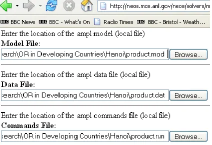
The NEOS server [Czyzyk et al 1998, www-neos.mcs.anl.gov,] is

open and free to the public for the optimization of large models within certain time or solver-dependent iteration limits. A user submits online a model specified in one of the input formats accepted by a solver (such as AMPL), a data set and a run file as shown in Figure 1.

Figure 1: Example of a NEOS input screen.

14

of solvers, but not all take input from AMPL. One which does is MINTO [coral.ie.lehigh.edu/minto], but it is slower than CPLEX.

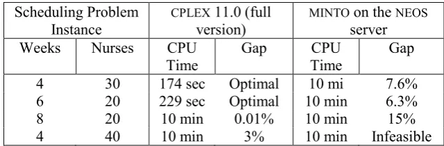
Clark and Walker (2008) used both CPLEX 11.0 and MINTO to solve an integer linear programme that allocates 20 nurses to 26 pre-selected shift patterns to provide cover for three shifts a day over 28-day. CPLEX 11.0 took 0.23 seconds to find an optimal zero-valued solution, i.e., all 20 nurses’ shifts fitted requirements exactly with no shortages or surpluses. The MINTO solver on the NEOS server took only a little longer at 1.62 seconds. Under tighter conditions that require cover by an extra nurse in each shift, CPLEX took 33 seconds to an optimal non-zero-valued solution as a schedule. Imposing a maximum solution time of 10 minutes, MINTO used up all this time, finishing with a solution that was within 17% of optimality. Table 1 shows the results obtained when scaling up the problem size under tight conditions. Observe that a quality commercial solver such as CPLEX can give near-optimal solutions for large realistically-sized instances, while MINTO on the NEOS server clearly struggles and would require alternative solution methods or decomposition into smaller problems.

Scheduling Problem Instance

CPLEX 11.0 (full

version)

MINTO on the NEOS

server

Weeks Nurses CPU

Time

Gap CPU

Time

Gap

4 30 174 sec Optimal 10 mi 7.6%

6 20 229 sec Optimal 10 min 6.3%

8 20 10 min 0.01% 10 min 15%

4 40 10 min 3% 10 min Infeasible

Table 1: Results after scaling up under tight conditions

3.6 COIN-OR

15

This is achieved by using the open-source solver CLP of the Computational Infrastructure for Operations Research (COIN-OR) project [coin-or.org], an initiative to spur the development of

open-source software for the OR community. The development effort in the C programming language, can be substantial as the CLP model data have to be jointly specified element by element in the unfriendly MPS format, a time-consuming task requiring detailed attention. Thus CLP is not suitable for prototyping, but rather for stable models.

COIN-OR also includes many other optimisation tools. including the CBC branch-&-cut solver that is available as a library or standalone solver, as well as on NEOS, using MPS or AMPL input.

4. CONCLUSION

This article has shown that sophisticated decision-making technology is available to persons and organisations worldwide without having to purchase expensive optimisation software. The use of such technology often involves the judicious combination of tools from disparate sources, but usually not in the seamless manner that a lay-user desires. It does requires competence, confidence and patience in the use of the internet, a little command-line programming, and text file editing, being qualities possessed by most technically competent persons.

5. REFERENCES

Caulkins J P, Morrison E L, Weidemann T (2007). Spreadsheet Errors and Decision Making: Evidence from Field Interviews. Journal of Organizational and End User Computing, 19: 1-23. Clark A R, Walker H (2008). Nurse Rescheduling, 18th Triennial Conference of the International Federation of Operational Research Societies, Johannesburg. 13-18 July 2008. Available online at http://tinyurl.com/ojhm3e.

16

Elizandro D , Taha H (2007). Simulation of Industrial Systems: Discrete Event Simulation Using Excel/VBA. Auerbach Publications.

Finlay P N, Wilson J M (2000). A survey of contingency factors affecting the validation of end-user spreadsheet-based decision support systems. Journal of the Operational Research Society 51: 949-958.

Grossman T A (1997). End-user modeling. OR/MS Today,

24(5).

Hillier F A (2009). Introduction to Operations Research. 9th ed., McGraw-Hill.

Linderoth J T, Ralphs T K (2005).Noncommercial Software for Mixed-Integer Linear Programming. In Integer Programming: Theory and Practice. John Karlof (ed), CRC Press Operations Research Series. pp 253-303.

Markham I S, Palocsay S W (2006). Scenario Analysis in Spreadsheets with Excel's Scenario Tool, Informs Transactions on Education. 6(2), 23-31. Available online at http://ite.pubs.informs.org/.

Martin A (2000). An integrated introduction to spreadsheet and programming skills for operational research students. Journal of the Operational Research Society 51:1399-1408.

Powell S G (1997). End-user modeling. OR/MS Today, 24(4). Taha H A (2008). Operations Research: An Introduction. Pearson,

Taube M (1996). Integrated Planning for Poultry Production at Sadia. Interfaces, 26: 38-53.

Zhu J (2008). Quantitative Models for Performance Evaluation and Benchmarking - Data Envelopment Analysis with Spreadsheets. 2nd Edition, Springer.

Weintraub A C, Church R L C, Murray A T C, Guignard M C (2000). Forest management models and combinatorial algorithms: analysis of state of the art. Annals of Operations Research, 96: 271-285.