whitepaper Benchmarking Jun2011 v2

Creating Land Surface Temperature Datasets for Validation and

Assessment of Homogenisation Algorithm Performance

1

Kate Willett, 2Claude Williams, 3Ian Jolliffe, 4Robert Lund, 5Lisa Alexander, 6Olivier Mestre, 7Stefan Brönnimann, 8Lucie Vincent, 9Steve Easterbrook, 10Victor Venema & 2

Peter Thorne

1

Met Office Hadley Centre, FitzRoy Road, Exeter, UK 2

National Climatic Data Center, Ashville, NC, USA 3

University of Exeter, Exeter, UK 4

Department of Matematical Sciences, Clemson University, SC, USA 5

Climate Change Research Centre, University of New South Wales, Australia 6

Meteo France, France 7

University of Bern, Switzerland 8

Climate Research Division, Science and Technology Branch, Environment Canada, Canada

9

Department of Computer Science, University of Toronto, Canada 10

Meteorologisches Institut, University of Bonn, Germany

1. Introduction:

Monitoring and understanding our climate requires robust assessment of means, trends and variability of ambient temperatures representative of a point in space that are free from any non-climatic influences. Ensuring station homogeneity in the absence of complete and verified metadata is very difficult; many algorithms exist with varying strengths, weaknesses and levels of skill (e.g., Peterson et al. 1998; Reeves et al. 2007). This leads to large methodological uncertainty between data-products. Verifying individual method skill is impossible because the absolute ‘truth’ is always unknown. Synthetic datasets where the 'truth' is known and errors are then added enable such assessment. However, the ability to achieve true homogeneity has rarely been comprehensively assessed for truly real world conditions.

Real observational data contain both low frequency and high frequency 'noise' (natural variability and random error). Discontinuities may be: geographically or temporally clustered; close to end points; gradual; alter the variance; in the presence of a long-term background trend; small; frequent; seasonally or diurnally varying; or all of the above. Identifying the correct time and magnitude for any discontinuity against background noise is difficult, especially if discontinuity magnitude varies diurnally and seasonally. Even after detection a series of decisions are required as to whether and how to adjust. These can have a further non-negligible impact upon the resulting dataset estimates. While decisions are as evidence-based as possible, some are unavoidably arbitrary. This is especially problematic for large datasets where the whole process by necessity is automated.

It is desirable to benchmark homogenisation methodologies by testing them on

fully capture real world noise and errors as described above. Recent studies (e.g., Menne & Williams 2005; DeGaetano 2006; Wang et al. 2007 and Wang et al. 2008a; 2008b; Titchner et al. 2009) have generated synthetic data test cases with varying degrees of real world characteristics (e.g. variance, autocorrelation and randomly assigned sign or position of discontinuity) or re-sampled real-data series that are known to be homogeneous (e.g. bootstrap; Wang et al. 2010).

At present, no agreed global standard exists against which to benchmark multiple datasets. Worse still, existing benchmark data are usually created by the dataset creators themselves leaving potential for intentional or unintentional tuning of algorithms to specific test cases. The issue is becoming increasingly critical, where policy decisions of enormous societal and economic importance are now being based on conclusions drawn from observational data. In addition to underpinning our level of confidence in the observations, developing and engendering a comprehensive and internationally recognised benchmark system will have three key scientific benefits:

o objective intercomparison of data-products

o quantification of structural uncertainty of any one product o a valuable tool to advancing algorithm development

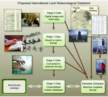
Here we describe the development of synthetic test data, assessment techniques and a programme cycle within which to operate. The benchmark analog data are to be part of the Surface Temperature Initiative (www.surfacetemperatures.org, Thorne et al. 2011 submitted to BAMS) databank as shown in Fig. 1. They will use the format and structure of the consolidated master database/stage 3 data in the databank such that the

benchmark analogs will represent, for the most part, the actual station compilation within the databank (section 2.1). As the databank may contain 60 000+ stations this actually means a sufficient proportion with which to constitute global coverage. There will be analog-known-worlds, each containing a homogenous set of analog-stations as described in section 2.2. There will then be 8 analog-error-worlds, each

presenting a different suite of discontinuity test cases (section 2.3 and 2.4) that originate from an analog-known-world. Essentially, a perfect homogenisation algorithm would adjust any analog-error-world to match the analog-known-world. In reality we are assessing the degree to which any algorithm is successful.

The key areas of effort are described in detail below:

i. Using GCMs as source data for analog-world construction ii. A model for creation of analog-known-world truth iii. Model for creation of analog-error-worlds

iv. Exploring all eventualities with optimum discontinuity test case design v. Assessment of performance against the benchmarks

vi. The benchmarking cycle

2. Approaches for Creating Temperature Benchmarking Datasets

2.1 Using GCMs as source data for analog-known-world construction

and natural variability), station autocorrelation and interstation characteristics, sampling density (network coverage and missing data) and presence of a long-term background trend). Hence, a true test of algorithm skill requires global reconstruction of real world characteristics including space and time sampling of the observational network as far as possible. Analog-known-world data should be created at a range of resolutions (sub-daily to monthly) with identical underlying characteristics. This will be particularly relevant to those groups considering temporal transferability of algorithms. For the first cycle we will concentrate on the monthly timescale.

Global Circulation Models can provide the majority of features described above albeit for gridded fields. Many of these include volcanic and solar forcings, represent modes of variability (e.g., ENSO) adequately including teleconnections and include various levels of anthropogenic forcings (from none [natural forcings only] through to high emissions scenarios) which essentially govern long-term changes. It is feasible to downscale a selection of model runs from the grid-box to match a given global station network spatially and temporally. Nudges can be made to each analog-station

climatology, variance and white noise characteristics to reflect real world attributes of that particular station (Fig. 2) – station autocorrelation and interstation relationships should be maintained as far as possible. Where possible, efforts should collaborate with and build on existing work such as that undertaken by the COST HOME project.

2.2 A model for creation of an analog-known-world with climatic possible patterns of perturbation

As described above, the analog-known-world needs to incorporate real world characteristics of the global observing network but be homogeneous so that the mean state characteristics (climatology, variance etc.) and any background trends are ‘knowns’. A simple model has been devised to quantify this:

X

= S

+ T

+

Σ

where t is time and l is location in (latitude, longitude and elevation) – there may be missing data in any station time series. X is the station observation which will have a real world identifier (e.g., WMO, WBAN etc.) used for its real station equivalent. S is any diurnal or seasonal cycle relevant to that particular station for that time and location. T is any background trend which includes: long term change signals; modes of variability (i.e., ENSO, NAO, PDO etc.); volcanic forcings; and solar forcings). _Σ is the remaining white noise randomness and error in the observations – even after rigorous quality control there is likely to be some error remaining in addition to some high frequency variance related to micro-climate and its manifestations of synoptic scale events. Maintaining real world interstation characteristics is essential and can be done using downscaling methods and information from the actual databank stations.

2.3 A model for creation of analog-error-worlds with non-climatic possible patterns of perturbation

X

= S

+ T

+

Σt,l

+ D

These discontinuities are in essence deviations from the ambient air temperature representative for a given location. They should be physically plausible

representations of known causes of sustained deviation (e.g., station moves, instrument malfunctions or changes, screen/shield changes, changes to observing practice or time) as summarised in Table 1. They should take into account the effect on temperature from the change in radiation and windspeed as accurately as is

possible at present, accepting that in the current state of knowledge this will be largely an assumption based on expert judgement.

Discontinuities added should be both abrupt and gradual, including the effects of land use change (including rural-to-urban developments) which is important for some applications. They should explore changes that vary with season, time of day (when we eventually create sub-daily analogs), and possibly with background temperature. In effect, these will be changes to the variance. Some should be geographically common and others distinct – rural-to-urban changes can radiate erratically from localised areas. Some discontinuities are well documented and pinned to a period and region (i.e. mid-to-late-1980s MMTS conversion in the USA maximum and minimum temperature series) and these (or similar) could be included in one of the analog-error-worlds. However, far more are undocumented and unknown and could be of any magnitude, frequency, clustering or sign bias and are likely a combination of all and a mix of abrupt and more gradual discontinuities. They should explore a range of frequencies and magnitudes. A review paper is in preparation to summarise the current state of knowledge on causes of discontinuities in the land temperature record and how they affect the data at a range of scales.

Metadata will be made available digitally as we move forward into the future and a small amount is available for some stations already. This is a useful tool in detecting discontinuities. Therefore, some discontinuities should be documented, some should not be and some should have documented changes where no actual temperature change is effected to cater for users with methods that use metadata.

2.4 Exploring all eventualities with optimum error-world design

Eight global error-worlds should be designed in parallel with the three aims of this work in mind: to aid product intercomparison; to help quantify structural uncertainty; and to aid methodological advancement. They should range from overly optimistic (e.g., mostly a few large discontinuities in the mean) to overly pessimistic (e.g., many small and large discontinuities that are both abrupt and gradual, affect the mean and variance, with some that are geographically clustered) and lead to clear and useful results. This will distinguish strengths and weaknesses of algorithms against specific discontinuity characteristics without completely overloading them from the start with a multitude of complexities. Importantly, the ‘known’ truth and exact error model of each world should not be known by those testing their algorithms on it to prevent deliberate or accidental optimisation for specific error worlds.

and adjustments. Worlds should incorporate a mix of discontinuity types discussed above and the set of worlds should be broad, covering all possibilities as not to penalise or support any one type of algorithm. They should methodically address key questions by testing skill under these situations (e.g., discontinuity clustering verses sparsity; proximity to endpoints verses midpoints; large versus small discontinuities; a combination of both; and the presence of strong versus no background trend [i.e., taken from control, A1B, C20C and natural climate runs] etc.). This concept is shown diagrammatically in Fig. 3.

2.5 Assessment of performance against the benchmarks

The benchmark analog-error-worlds will be freely available in an identical

format/structure to the stage 3 database of the Surface Temperature Initiative databank (link when available). Data-product creators are strongly encouraged to run their homogenisation algorithms on the analog-error-worlds to create adjusted analog-error-worlds and submit results to the Benchmarking and Assessment Working Group for assessment. It is important that this process is made easy to encourage participation.

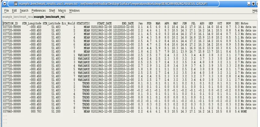
This could either be done by data-product-creators submitting algorithms and station selections to the data-product portal – this is associated with the Surface Temperature Initiative and is an online database hosting any product relating the databank (link when available). It would then be the responsibility of members of the Benchmarking and Assessment Working Group or Steering Committee to run that algorithm on the selection of stations given and produce the results that will be stored online with the data-product. Alternatively, the onus could be on the data-product creators to also download an identical station selection to that going into their product from each of the analog-error-worlds and run their algorithm on each. They would then submit a specified format ascii list of station, longitude, latitude, start date, end date, start magnitude, end magnitude (in case of gradual discontinuities) and characteristics (e.g., seasonal, variance, mean, etc.) for each discontinuity detected (Fig. 4). They would also be asked to submit station climatological means, variance and trends for each analog-error-world (Fig. 5). It would be the responsibility of the Benchmarking and Assessment Working Group to then perform the assessment using the methods outlined below. In time this process could be automated.

Assessment can be conducted in two ways: does it locate the discontinuities correctly; and does it apply the correct adjustment factor? These can be assessed both

and False Alarm Rate. Users can then quickly see which worlds that particular data-product/algorithm scores highly in and which worlds are problematic. This can be used to infer applicability of data-products for a specific use or intercomparison with data-products created from different algorithms.

Homogenisation algorithms that include adjustment will produce an estimate of large scale features (climatology, variance and trends) for each analog-error-world. A perfect algorithm would recreate the analog-known-world features across a range of space and time scales. Algorithms should, ideally, at least make the analog-error-worlds more similar to the analog-known-world. This information can be calculated for stations, regional means or global averages from each adjusted analog-error-world and ‘distance’ measured in terms of proximity in o C for mean and trends and standard deviation for variance and summarised graphically (Fig. 7). For example, a score between 0 and 2 could be used where: 0 is perfectly matching the analog-known-world features; 1 is having no useful skill as the features either remain identical to that of the analog-error-world or move it to the same distance beyond that of the analog-known world; and 2 is having terrible skill where the algorithm moves the analog-error-world at least the same distance away again or two times the distance beyond the analog-known-world.

At present all development efforts will focus on monthly mean data. Although

successful homogenisation of sub-daily or even daily resolution data has not yet been demonstrated the Surface Temperature Initiative will likely spur attempts at this and so the benchmarking programme needs to be available at high resolution.

2.6 The Benchmarking Cycle

The complete benchmarking process will be conducted in 3 year cycles, overseen by the Benchmarking and Assessment Working Group. It will consist of: concept development; creation of analog-known-world and analog-error-worlds; release of the analog-error-worlds and assessment of resulting data-products; later release of the analog-known-world; and finally a wrap-up with a workshop and analysis paper.

The concept development will be done by the whole Benchmarking and Assessment Working Group and published in a peer-reviewed paper. This will include release of an example set of benchmark analogs (analog-known-world and analog-error-worlds) to maximise the scientific benefit to those developing homogenisation algorithms and methods to address bias and uncertainty. Importantly, the creation of the specific features of the analog-known-world and analog-error-worlds for official release as part of the Surface Temperature Initiative databank should be done by a third party that does not include those likely to create data-products and use the

benchmark analogs. This retains the value of the actual discontinuities within the

analog-error-worlds being ‘unknown’ errors as in the real world.

analog-known-world, is unknown. Data-product creators will be encouraged to run their algorithms on whatever station subset of the analog-error-worlds they use for their

data-product. It will be the role of the Benchmarking and Assessment Working Group to advocate and support use of these benchmark analogs and also to perform the assessment on the resulting analog-products (section 2.5). Then, 2.5 years later the

analog-known-world will be released providing a new tool for algorithm developers and those working to quantify methodological uncertainty.

The wrap-up will bring together users and creators of the benchmark analogs to assess how they were useful and how they can be improved for the next cycle. This will likely be in the form of a workshop and overview analysis paper. The databank will develop over time as will algorithms and the benchmark analogs will need to update both in terms of station coverage and methodologically. An important step will be providing the benchmark analogs for higher resolution data and then for variables other than temperature. To ensure that this happens we intend to conduct the

benchmark development, creation, release of analog-error-worlds, release of the

analog-known-world and wrap up workshop and paper in three year cycles.

3. The Benchmarking and Assessment Working Group

The Benchmarking and Assessment Working Group was set up during the Exeter 2010 workshop for the Surface Temperature Initiative. It has now been populated by and international and interdisciplinary group of people. Its purpose is to develop and oversee the benchmarking process as described here. Further details can be found at www.surfacetemperatures.org/benchmarking-and-assessment-working-group and blog discussions can be found at http://surftempbenchmarking.blogspot.com. The Benchmarking and Assessment Working Group report to the Steering Committee and are guided by the Benchmarking and Assessment Terms of Reference hosted at www.surfacetemperatures.org/benchmarking-and-assessment-working-group.

To complete all the tasks laid out in this paper it is likely that three sub-groups will be formed. Group 1 would be responsible for designing and developing the analog-known-world(s). Group 2 would be responsible for devising and developing the

analog-error-worlds. Group 3 would be responsible for devising and developing the assessment system. Importantly, these three entities should not be devised in isolation and so communication between groups is essential to ensure consistency of purpose throughout. Furthermore, these groups are responsible for the initial development which should provide software to create future versions/perform assessments. This software can then be used by third parties who are able to alter parameters to create unique analog-known-worlds and analog-error-models for each cycle (although this system may need some level of development/advancement over time). This double-blind approach ensures that the ‘knowns’ remain truly hidden for each cycle.

Recommendations:

• Global analog-known-world data with real world characteristics • GCM data should be used as source base with real spatial, temporal and

climatological characteristics applied

• Suite of ~8 analog-error-worlds that are physically based on real world

discontinuities and orthogonally designed to maximise the number of objective science questions that can be answered

• Benchmarking to quantify algorithm skill in terms of performance using

climatology, variance and trends of the adjusted analog-error-worlds versus those of the analog-known-world(s) and an assessment of hit rates versus false alarm rates

• Independent (of any single group of dataset creators) analog-known-world(s)

and analog-error-worlds data creation with the analog-known-worlds and specific discontinuities applied the analog-error-worlds withheld until 6 months prior to the end of the benchmarking cycle

• Peer-reviewed publication of benchmarking methodology and initial release of

a set of analog-known-world(s) and analog-error-worlds

• A three year benchmarking cycle lagging formal databank updates by 6

months involving development and creation of new benchmark analogs, release of the analog-error-worlds, advocacy and support for users and assessment of results submitted, release of the analog-known-world(s) and finally a wrap-up workshop resulting in an analysis publication

References: 6

http://www.homogenisation.org 7

http://www.esrl.noaa.gov/psd/data/gridded/data.20thC_Rean.html 8

http://cmip-pcmdi.llnl.gov/cmip5/data_description.html?submenuheader=1

Begert, M., Zenklusen, E., Haberli, C., et al., 2008: An automated procedure to detect discontinuities; performance assessment and application to a large European climate data set. Meteorologische Zeitschrift. 17, (5), 663-672.

DeGaetano, A. T., 2006: Attributes of several methods for detecting discontinuities in mean temperature series. Journal of Climate. 19 (5), 838-853.

Ducré-Robitaille, J.-F., Vincent, L. A. & Boulet, G., , 2003: Comparison of

techniques for detection of discontinuities in temperature series. International Journal of Climatology, 23, 1087-1101.

Easterling, D. R. & Peterson, T. C., 1995: The effect of artificial discontinuities on recent trends in minimum and maximum temperatures. International Minimax Workshop on Asymmetric Change of Daily Temperature Range, SEP 27-30, 1993 COLLEGE PK, MD. Atmospheric Research. 37, 19-26.

Elliott, W. P., 1995: On detecting long-term changes in atmospheric moisture. International Meeting of Experts on Long-Term Climate Monitoring by the Global Climate Observing System, JAN 09-11, 1995 ASHEVILLE, NC. Climatic Change.

31, 349-367.

Menne, M. J. & Williams, C. N., 2005: Detection of undocumented changepoints using multiple test statistics and composite reference series. Journal Of Climate. 18,

Peterson, T. C., Easterling, D. R., Karl, T. R., et al., 1998: Homogeneity adjustments of in situ atmospheric climate data: A review. International Journal Of Climatology.

18, 1493-1517.

Titchner, H. A., Thorne, P. W., McCarthy, M. P. et al. 2009: Critically Reassessing Tropospheric Temperature Trends from Radiosondes Using Realistic Validation Experiments. Journal Of Climate.22, 465-485.

Vincent, L.A., 1998: A technique for the identification of inhomogeneities in Canadian temperature series. Journal of Climate, 11, 1094-1104.

Vincent, L. A., van Wijngaarden, W. A. & Hopkinson, R., 2007: Surface temperature and humidity trends in Canada for 1953-2005. Journal of Climate, 20, 5100-5113. DOI: 10.1175/JCLI4293.1.

Wang, X. L., Wen, Q. H., and Wu, Y., 2007: Penalized Maximal t Test for Detecting Undocumented Mean Change in Climate Data Series. Journal of Applied Meteorology and Climatology. 46, 916-931. DOI:10.1175/JAM2504.

Wang, X. L., 2008a: Accounting for autocorrelation in detecting mean-shifts in climate data series using the penalized maximal t or F test. Journal of Applied Meteorology and Climatology. 47, 2423–2444. DOI: 10.1175/2008JAMC1741.1

Wang, X. L., 2008b: Penalized maximal F test for detecting undocumented mean-shift without trend change. Journal of Atmospheric and Oceanic Technology, 25, 368-384. DOI:10.1175/2007/JTECHA982.1.

Figure 1 Structure of the Surface Temperature Initiative Databank

Figure 3 Example of a set of analog-error-world models

Figure 4 Example ASCII file containing discontinuity detections and adjustments for each station to be uploaded to the data-product portal for assessment by the Benchmarking and Assessment Working Group against the analog-known-world(s)

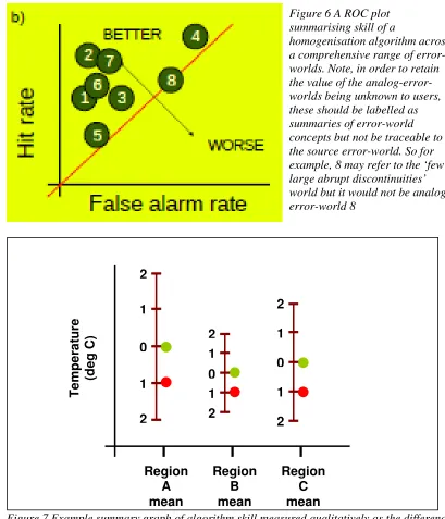
Figure 7 Example summary graph of algorithm skill measured qualitatively as the difference in climatological mean between an adjusted analog-error-world and the analog-known-world for different regions. Green dots represent the region mean temperature from the

analog-known-world. Red dots represent the region mean temperature from an analog-error-world. The numbered ladder (2 to 0 to 2) shows the algorithm score depending on where the region mean from the adjusted analog-error-world lies. It may lie beyond 2 and the scale could be continued indefinitely where 0 indicates a perfect algorithm, 0-1 indicates that the algorithm improves the data and 1+ indicates that the algorithm makes the data worse.

Figure 6 A ROC plot summarising skill of a

homogenisation algorithm across a comprehensive range of error-worlds. Note, in order to retain the value of the analog-error-worlds being unknown to users, these should be labelled as summaries of error-world concepts but not be traceable to the source error-world. So for example, 8 may refer to the ‘few large abrupt discontinuities’ world but it would not be analog-error-world 8

Region A mean

Region B mean

Region C mean

T

e

m

p

e

ra

tu

re

(d

e

g

C

)

0 2

1

1

2

0 2

1

1

2 0

2 1

Table 1. Known discontinuities between observed air temperature and the ambient air temperature representative of a given location in terms of: problems; possible causes and effects; physical solutions; and possible implementations in modelling a benchmark.

Problem Possible Cause Possible Effect Physical solution Benchmark modelling Reported air temperature is not measured air temperature Errors in reporting, units, etc.

Abrupt change that is either constant over time or a function of temperature

Identify error and correct (difficult to adjust using an automated process

because errors may be unique)

Draw from past experience. Apply blanket changes using a constant or simple formula as a

function of temperature alone

Measured air temperature is

not true air temperature

Instrument error (malfunction or change in type), calibration error

Abrupt (or gradual for some instrument malfunctions) change that is either constant or a function of temperature

(or drifting for some instrument malfunctions) [random errors should be removed by quality control process]

Identify error and correct, using metadata where available

Statistically model distributions of typical size and frequency. Apply blanket changes using a constant or simple formula as a function of

temperature alone True air temperature is not representative ambient air temperature Change in instrument shield, practice or microclimate (due to move of

instrument)

Abrupt change that is likely to vary as a function of variables such as radiation,

windspeed and soil moisture

Identify error and correct. Modelling energy balance of shield and

microclimatic conditions

Statistically model distributions of typical size and frequency. Semi-empirical modelling of errors based on assumed changes in radiation,

windspeed and soil moisture.

Representative ambient air temperature is affected by local influences Changes in station surroundings, urbanization

Gradual change that is likely to vary as a function of variables such as radiation, windspeed and soil moisture

Correction not desirable from a physical or monitoring perspective, but

from a detection and attribution perspective. Modelling energy balance of shield and microclimatic conditions

Statistically model distributions of typical size and frequency. Semi-empirical and possibly numerical modelling of resulting trend and its high frequency characteristics due to changes in

radiation, windspeed and soil moisture.

Different ambient air temperatures are

merged

Change in station location

Abrupt change that is likely to vary as a function of variables such as radiation,

windspeed and soil moisture

Unmerge (correction not desirable from a physical perspective, especially for

high frequency data, but from a low frequency large scale monitoring and detection and attribution perspective)

Change in spatial sampling from the analog-known-world to merge series.

Changes in diurnal sampling affect statistics Change in observation time

Abrupt change that is likely to vary as a function of variables such as radiation

Correction not desirable from a physical perspective, but from a low frequency large scale monitoring and detection and attribution perspective

Statistically model distributions of typical size and frequency. Change in temporal sampling from synthetic source data or in the case of low

frequency GCM output use semi-empirical modelling of errors based on assumed changes

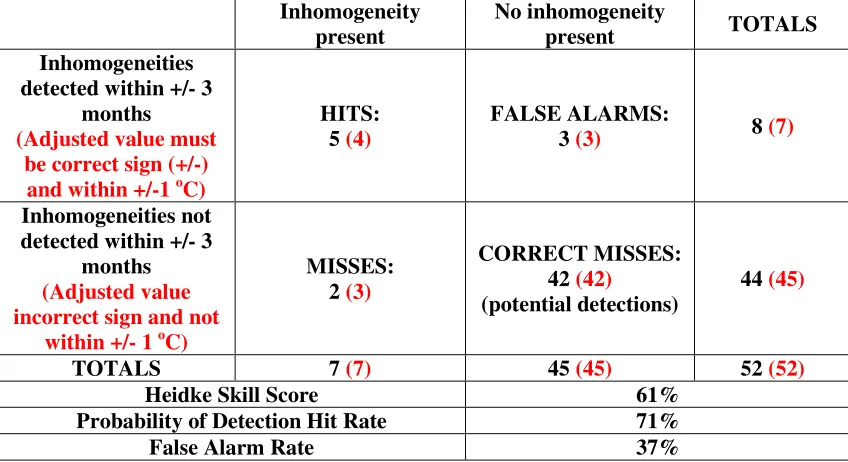
Table 2 Example contingency table for assessing detection and also adjustment (option shown in red) skill of homogenisation algorithms. Potential detections are the number of potential discontinuities within the time period minus the total number of detections and misses. These are used to quantify those occasions where no discontinuity is found and none is present. This is done by assuming that there is potentially a maximum of 1 discontinuity every 6 months (some algorithms can only search for discontinuities with 6 months of data either side) such that a 26 year period will have 52 potential discontinuities.

Inhomogeneity present

No inhomogeneity

present TOTALS

Inhomogeneities detected within +/- 3

months (Adjusted value must

be correct sign (+/-) and within +/-1 oC)

HITS: 5 (4)

FALSE ALARMS:

3 (3) 8 (7)

Inhomogeneities not detected within +/- 3

months (Adjusted value incorrect sign and not

within +/- 1 oC)

MISSES: 2 (3)

CORRECT MISSES: 42 (42) (potential detections)

44 (45)

TOTALS 7 (7) 45 (45) 52 (52)

Heidke Skill Score 61%

Probability of Detection Hit Rate 71%