www.biogeosciences.net/11/5087/2014/ doi:10.5194/bg-11-5087-2014
© Author(s) 2014. CC Attribution 3.0 License.
Causal relationships versus emergent patterns in the global
controls of fire frequency
I. Bistinas1, S. P. Harrison2,3, I. C. Prentice3,4, and J. M. C. Pereira1
1Forest Research Centre, School of Agriculture, University of Lisbon, Tapada da Ajuda 1349–017 Lisbon, Portugal 2Geography and Environmental Sciences, School of Archaeology, Geography and Environmental Sciences (SAGES),
Reading University, Whiteknights, Reading, RG6 6AB, UK
3Department of Biological Sciences, Macquarie University, North Ryde, NSW 2109, Australia
4AXA Chair of Biosphere and Climate Impacts, Grantham Institute for Climate Change and Grand Challenges in Ecosystems
and the Environment, Department of Life Sciences, Imperial College London, Silwood Park Campus, Buckhurst Road, Ascot, SL5 7PY, UK
Correspondence to: I. Bistinas ([email protected])
Received: 31 January 2014 – Published in Biogeosciences Discuss.: 7 March 2014 Revised: 25 June 2014 – Accepted: 19 August 2014 – Published: 22 September 2014
Abstract. Global controls on month-by-month fractional burnt area (2000–2005) were investigated by fitting a gen-eralised linear model (GLM) to Global Fire Emissions Database (GFED) data, with 11 predictor variables repre-senting vegetation, climate, land use and potential ignition sources. Burnt area is shown to increase with annual net primary production (NPP), number of dry days, maximum temperature, grazing-land area, grass/shrub cover and diurnal temperature range, and to decrease with soil moisture, crop-land area and population density. Lightning showed an appar-ent (weak) negative influence, but this disappeared when pure seasonal-cycle effects were taken into account. The model predicts observed geographic and seasonal patterns, as well as the emergent relationships seen when burnt area is plot-ted against each variable separately. Unimodal relationships with mean annual temperature and precipitation, population density and gross domestic product (GDP) are reproduced too, and are thus shown to be secondary consequences of correlations between different controls (e.g. high NPP with high precipitation; low NPP with low population density and GDP). These findings have major implications for the design of global fire models, as several assumptions in current mod-els – most notably, the widely assumed dependence of fire frequency on ignition rates – are evidently incorrect.
1 Introduction
appropriate management strategies and land-use policies can be developed (e.g. Moritz et al., 2012; Amatulli et al., 2013). The availability of remotely sensed data in a number of ac-tive fires (Giglio et al., 2006; Bartlein et al., 2008) and burnt areas (Giglio et al., 2010) during the past decade makes it possible now to analyse the controls on wildfire on a global scale (Krawchuk et al., 2009; Aldersley et al., 2011; Da-niau et al., 2012; Moritz et al., 2012; Knorr et al., 2014). Each of these studies considered different sets of potential controls and used different methods. Krawchuk et al. (2009) (updated by Moritz et al., 2013) used generalised additive models (GAMs) to explore relationships between burnt area and 17 climate variables, net primary production and two measures of human impact. Different subsets of variables were selected by individual GAMs, but the availability of fuel (quantified by net primary production, NPP) was the strongest single predictor in all cases. Aldersley et al. (2011) used a regression-tree and random-forest approach to exam-ine the influence of climate, vegetation and human impact on burnt area. Climate and climate-determined vegetation prop-erties were the most important controls. Knorr et al. (2014) examined human impact on annual burnt area using non-linear models, which show that the dominant influence of hu-mans on a global scale is to reduce fire frequency. Statistical models have been used to predict the potential consequences of future climate change for fire regimes (Krawchuk et al., 2009; Moritz et al., 2012). We suggest that the reliability of these predictions depends on the degree to which the fitted statistical relationships reflect underlying processes.
Process-based fire modules have also been developed and included in dynamic global vegetation models (DGVMs), but current DGVMs differ greatly in the processes they con-sider and how they are represented. Some models (e.g. LPJ-SPITFIRE: Thonicke et al., 2010; LPJ-LMfire (v1.0): Pfeif-fer et al., 2013; CLMfire: Kloster et al., 2010; Li et al., 2012) have included human ignitions as a right-skewed unimodal function of population density, with ignitions increasing up to an optimum population density and decreasing thereafter. In contrast, the LPX model (Prentice et al., 2011; Kelley et al., 2014) considers only ignitions caused by lightning. Some models include the effects of land use by suppressing fire in cropland areas (e.g. LPX) and/or reducing fuel loads on grazing lands (e.g. ORCHIDEE: Krinner et al., 2005; Chang et al., 2013). None of these treatments is based on extensive data analysis.
Both the global consequences and the regional predictions of future fire hazards vary considerably between models and different types of models (Harrison et al., 2010). Krawchuk et al. (2009) showed increased future fire in boreal forests, while simulations with fire-enabled dynamic global vegeta-tion models (DGVMs) have shown a decrease (Scholze et al., 2006), an increase (Kloster et al., 2010) or no change (Harri-son et al., 2010). We infer that the present level of scientific understanding of fire, as embodied in current models, is low.
Here we adopt a hybrid approach that is observationally based, but with the choice of environmental predictor vari-ables guided by explicit hypotheses about the potential con-trols of a burnt area. We focus on burnt area, as (a) it is a general measure of the ecological and human importance of fire – equivalent to fire frequency, i.e. the probability of fire per unit time at a randomly chosen point in space (Knorr et al., 2014) – and (b) it is a key determinant (along with biomass) of the emissions of atmospheric constituents that influence climate, including greenhouse gases, volatile organic compounds and black carbon (Arneth et al., 2010). We use a generalised linear model (GLM) to relate the frac-tional burnt area to a series of predictors representing the po-tential vegetation, climatic and human controls on fire igni-tion and spread. GLM modelling has previously been used by Lehsten et al. (2010) to model burnt area in Africa.
A key point in our analysis is the distinction between “un-derlying” relationships (fitted using statistical methods mak-ing the simplest possible assumptions about their form, and displayed using partial residual plots) and “emergent” pat-terns, which are observed when plotting burnt area against each variable by itself. Built-in partial correlations between the predictor variables ensure that the two kinds of plots ap-pear very different, and that the single-variable plots are not a reliable guide to the underlying relationships. To take one example that is already well understood (van der Werf et al., 2008; Harrison et al., 2010; Prentice et al., 2011), the emer-gent global relationship between burnt area and precipitation is unimodal, because fire is limited by fuel availability in dry climates, and by fuel moisture in wet climates. In other words, the underlying causes can be represented as a mono-tonically increasing relationship of fire probability with pri-mary production, and as a monotonically decreasing relation-ship with climatic moisture. The emergent unimodal pattern results from the combination of two different mechanisms by which precipitation controls vegetation and fuel proper-ties. We will demonstrate further examples where emergent unimodal responses of burnt area arise through the combined effects of different causal factors.
2 Data and methods
2.1 Generalised linear modelling
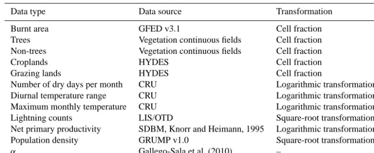
Table 1. Sources of data.
Data type Data source Transformation
Burnt area GFED v3.1 Cell fraction
Trees Vegetation continuous fields Cell fraction
Non-trees Vegetation continuous fields Cell fraction
Croplands HYDES Cell fraction
Grazing lands HYDES Cell fraction
Number of dry days per month CRU Logarithmic transformation
Diurnal temperature range CRU Logarithmic transformation
Maximum monthly temperature CRU Logarithmic transformation
Lightning counts LIS/OTD Square-root transformation
Net primary productivity SDBM, Knorr and Heimann, 1995 Logarithmic transformation
Population density GRUMP v1.0 Square-root transformation
α Gallego-Sala et al. (2010) –
for the use of a generalised linear model (GLM), of which ordinary least-squares regression is a special case. There is no standard method for handling quantitative data of this particular type in a GLM context. However, the GLM vari-ant known as logistic regression gives highly interpretable results with this kind of data (Wang et al., 2013). Logis-tic regression fits an underlying relationship between logit-transformed probability (y) and a linear combination of pre-dictors:
ln[y/(1−y)] =b0+b1×1+b2×2+... (1)
whereb0is the intercept andbiare the slope coefficients for
each variablei. In classical logistic regression, the data con-sist of ones and zeroes, and it is assumed that the data are bi-nomially distributed. The use of fractional data implies max-imisation of a quasi-likelihood function instead of a true like-lihood (Papke and Wooldringe, 1996). Implicitly, the burnt area data are treated as estimates of an underlying probabil-ity. The logarithm on the left-hand side of Eq. (1) implies that the predictors are assumed to combine multiplicatively, so the model is “linear” only in the sense that the terms on the right-hand side are added together.
Logistic regression was implemented using the GLM package in R. Goodness-of-fit of the complete model was quantified using the proportion of explained deviance, also known as McFadden’s R2(McFadden, 1974). This is a so-called pseudo-R2that can be interpreted analogously to the coefficient of determination in ordinary regression. Partial residual plots were used to display the fitted underlying re-lationship between each variable and the predicted probabil-ities. These plots are analogous tox–y plots in bivariate re-gression, except that they coordinate of each data point in each plot is shifted so as to remove the fitted partial effects of all the other predictors (Larsen and McCleary, 1972).z val-ues (slope coefficients normalised by their respective stan-dard errors) were used to quantify the importance of each partial relationship.zvalues are the most appropriate statis-tics for this purpose, because they express the strength of the
signal relative to noise, and are independent of the units of measurement. We did not include any interactions between predictors, nor did we add quadratic terms or use the more flexible functions represented by GAMs. Instead, we set out to discover whether key features of the burnt area data could be described adequately by a combination of independent, monotonically increasing (or decreasing) functions of the predictors.
2.2 Burnt area data
Global fractional burnt area data, on the standard 0.5◦grid, were obtained for each month from January 2000 to Decem-ber 2005, from the third version of the Global Fire Emissions Database (GFED3: Giglio et al., 2010). We confined our at-tention to the post-2000 period, for which the GFED data were derived by combining MODIS satellite observations with biome-dependent modelling of the relationship between burnt area and observed fires. We do not analyse the pe-riod post-2005, because other data sets (e.g. net primary pro-duction, NPP) are lacking. However, since we are consider-ing spatial relationships between burnt area and the predic-tor variables using monthly burnt area, this 72-month time period is adequate for diagnosing the key relationships. We made no attempt to screen the data for deforestation or agri-cultural fires, in part because of the difficulty in unambigu-ously identifying such fires, and in part because it is clear that the extent and timing of deforestation and agricultural fires are influenced by climatic factors (e.g. van der Werf et al., 2010). The fourth version of the GFED data became avail-able after our analyses were completed; we have checked that the results do not change when the newer data set is used.
2.3 Environmental predictor variables
varying (not varying between months), seasonally varying (not varying between years), and dynamic (varying between months and years).
Tree cover and grass/shrub cover: the division into forested and non-forested vegetation types is fundamental, distinguishing ecosystem types (e.g. forest versus savan-nas) and layers (canopy, subcanopy, ground cover) that can possess very different fire regimes (Lavorel et al., 2007). Brovkin et al. (2012) showed that woody litter decays an order of magnitude more slowly than grass litter. Frac-tional cover data (static) for trees and non-trees (defined as plants less than 5 m tall, whether shrubby or herbaceous) were obtained from the remotely sensed Vegetation Con-tinuous Fraction data set derived from MODIS (DeFries and Hansen, 2009). The two variables are not mutually re-dundant, because the data set also includes fractional bare ground.
Net primary production: fuel limitation is a major con-straint on burnt area (van der Werf et al., 2008). We used annual net primary production (NPP) (annually varying) as an index of the potential natural fuel load. NPP was included as annually varying because litter mass accumulates over a year or longer; it does not vary with monthly NPP. Annual NPP was estimated using the Simple Diagnostic Biosphere Model (SDBM, Knorr and Heimann, 1995), driven by re-motely sensed “greenness” (fractional absorbed photosyn-thetically active radiation) from the SeaWiFS data set (Go-bron et al., 2006). The SDBM is an implementation of the general light-use efficiency model for primary production. It provides the most accurate available gridded NPP data, as shown by its ability to predict observed seasonal cycles of CO2 concentration at different locations, so far unmatched
by any other model (Kelley et al., 2013), as well as field-based NPP where this has been measured.
Land use: human activities have greatly modified natural vegetation in much of the world (Sanderson et al., 2002). Intensive agriculture leads to landscape fragmentation (Guyette et al., 2002; Syphard et al., 2009), which inhibits fire spread by disrupting fuel continuity. Grazing also re-moves fuel, but fire has been used as part of the management of both croplands and grazing lands (Pyne, 2012; Fernan-des et al., 2013). Fractional cover data for crops and graz-ing land (static) were obtained from Vegetation Continuous Fields data set MOD44B (DiMiceli et al., 2011).
Climate: fuel dryness determines whether ignition events lead to spreading fires, and also the rate of spread and thus the area burnt. The Nesterov index (Nesterov, 1949) is one of the measures used to assess the risk of fire that takes into account factors that control drying rate. We selected climatic predictors based on the logic of the simplified Nesterov index used in the LPJ-SPITFIRE (Thonicke et al., 2010) and LPX (Prentice et al., 2011) models:
NI=XTmax·(Tmax−Tdew) (2)
where NI is the simplified Nesterov index,Tmaxis the daily
maximum temperature, Tdew is the dewpoint temperature
(approximated by the daily minimum temperature), and sum-mation is over each period of consecutive dry days, conven-tionally defined as days with 3 mm precipitation or less. The predictors used here are the monthly mean diurnal temper-ature range (a proxy for vapour pressure deficit), monthly mean daily maximum temperature, and the number of dry days in the month (ndry). Vapour pressure deficit is the main
environmental control on the drying rate of dead fuel. Diur-nal temperature range and maximum daily temperature de-termine flammability on a given day, but the time since rain is crucial for the evolution of fuel moisture. Dry days were entered as the rationdry/(1−ndry), which is proportional to
the expected time since a rainfall event. These three predic-tors are combined multiplicatively in the model, as they are in the index. Climate data were obtained from the Climate Research Unit (CRU) TS 3.1 time series data set.
Soil moisture: the moisture content of living fuel, and the rate of conversion to dead fuel in the case of grasses, is de-termined by soil moisture, which varies much more slowly through the season than either vapour pressure deficit or fuel moisture because the water-holding capacity of soil allows moisture to be retained for several months. Unfortunately, there is no reliable global data set of soil moisture. We there-fore used the ratio of actual to equilibrium evapotranspiration (α), which is widely used as an index of plant-available mois-ture (Prentice et al., 1993), as a surrogate for soil moismois-ture. This index is calculated from the CRU TS3.1 climate data as described in Gallego-Sala et al. (2010). Equilibrium evap-otranspiration refers to the water loss from a large homoge-neous area under constant atmospheric conditions. Estimated actual evapotranspiration depends on the rate of supply of moisture from the soil, which declines in proportion to soil water content.
population data, given that that it is difficult to test the re-alism of such redistribution. The resolution of the GRUMP data set is sufficient for our analyses over most of the globe, but the large size of some administrative units, for example in northern North America, could lead to slight biases in the assessment of the impact of humans on ignitions.
Some predictors used in previous analyses are not included in ours. Wind speed influences the rate of fire spread (Rother-mel, 1972; Weise and Biging, 1997), and is an important con-trol on the area burnt by any particular fire. We do not expect it to be important for monthly data at 0.5◦resolution. In any case, there is no reliable global data set for wind speed near the surface. Reanalysis products underestimate diurnal vari-ability in wind speed and gustiness (Sheridan, 2011), both of which are critical for fire spread. Gross domestic prod-uct (GDP) has been used as an index of cultural influences on the use of fire (Aldersley et al., 2011). The only avail-able global data set (http://sedac.ciesin.columbia.edu/data/ collection/gpw-v3) expresses GDP per unit area (rather than per capita), and is dominated by patterns in population den-sity. The primary data appear to have been collected either at country level or from variably sized administrative units. When population density is factored out (in order to estimate GDP per capita), the resulting mapped patterns are grossly unrealistic.
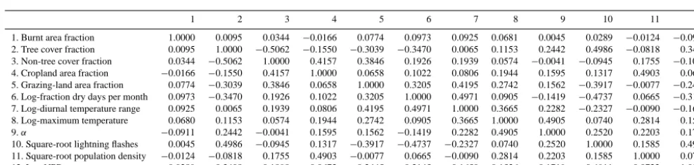
Many additional climate variables have been used in fire studies (see e.g. Krawchuk et al., 2009). These are expected to be highly correlated with other climate predictors, and less easy to relate mechanistically to fire properties. We wished to avoid inclusion of redundant variables to avoid multi-collinearity. We examined our set of predictor variables (Ta-ble 1) for independence using cross-correlation analysis. No pairwise correlation exceeded 0.5. Correlation among pre-dictor variables increases the sample size required to achieve statistical significance (Maxwell, 2000), but does not com-promise the validity of the regression coefficients or their estimated significance levels. By defining the combinations of predictors a priori we avoided the bias towards signifi-cance that is characteristic of stepwise methods (Cohen et al., 2003). The great majority of fires are much smaller than a grid cell, so there is effectively no contagion. Spatial auto-correlation is thus not a problem for this analysis as the data points can be considered as independent realisations of the underlying process.
Many of the predictor variables have highly skewed distri-butions. We transformed the data prior to analysis to reduce their skewness (Table 1). We used logarithmic transformation in cases where logically we expect there to be no fire when the predictor variable takes the value zero, and square-root transformation where this is not the case. If a log-transformed variable appears as one of thexiterms on the right-hand side
of Eq. (1), this is equivalent to fitting a power function (xi
raised to powerbi) in the multiplicative model. We made no
attempt to optimise the overall fit of the GLM model, and we use this final model to predict the probability of burnt area.
We carried out a further analysis in which pure seasonal-cycle effects were included. Two (seasonally varying) pre-dictors were added, namely sinθ and cosθ where January (in the Northern Hemisphere) or July (in the Southern Hemi-sphere) is coded asθ=0, and subsequent months in incre-ments ofπ/6. Positive (negative) values of sinθ represent proximity to spring (autumn), and positive (negative) values of cosθrepresent proximity to winter (summer). Each month possesses a unique combination of values of these two vari-ables.
We applied the GLM to predict seasonal burnt areas for 2005 as an example to demonstrate the realism of its spa-tial patterns, in comparison with maps based directly on the data. We also show the predicted emergent relationships of the modelled burnt area with each predictor, one by one, for comparison with similar plots derived directly from the data. The GLM can be used to predict emergent relationships with variables other than the selected predictors (i.e. differ-ently transformed, or even variables that were not included in the model). We examined the predicted and observed emer-gent relationships with mean annual temperature, mean an-nual precipitation, and the logarithms of population density and GDP.
3 Results
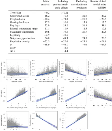
The fitted GLM attained a pseudo-R2 of 0.74. All the pre-dictor variables except tree cover were significant prepre-dictors of burnt area (Table 2). The strongest effects were an in-crease in burnt area with NPP (z=56.8), and a decrease in burnt area with soil moisture (z= −58.9). In addition, dry days (z=32.9), maximum temperature (z=19.6), grazing-land area (z=17.9), grass/shrub cover (z=16.2) and diur-nal temperature range (z=11.1) increased burnt area; hu-man population (z= −22.5) and cropland area (z= −22.0) decreased burnt area. These relationships were highly sig-nificant (P< 0.001). Partial residual plots (Fig. 1) show the fidelity of the data to the fitted relationships for these vari-ables. A general finding, however, is that some grid cells and months have exceptionally high burnt areas, not accounted for by the GLM, and thus appearing as a spread of large resid-uals above the fitted partial relationships.
Table 2. Regression coefficients from each of the three models. Non-significant values (P> 0.05) in parentheses.
Initial Including Excluding Results of final
analysis pure seasonal- non-significant model using
cycle effects predictors GFED4
Tree cover −0.2 (−0.1) – –
Grass/shrub cover 16.2 16.3 22.9 23.2
Cropland area −20.4 −19.8 −20.7 −20.5
Grazing-land area 17.9 16.6 17.9 17.5
Dry days 32.9 28.2 36.9 38.6
Diurnal temperature range 11.1 11.9 11.3 10.1
Maximum temperature 19.6 19.5 20.7 20.6
Lightning −2.9 −0.6 – –
Net primary production 56.8 49.3 74.3 73.6
Population density −22.5 −22.6 −23.1 −24.4
α −58.9 −46.1 −66 −64.4
cosθ – −8.5 – –
sinθ – −4.4 – –
Tree cover fraction
f( T re e c o v e r fr a c ti o n ) f(n o n -T re e c o v e r fr a c ti o n )
non-Tree cover fraction
f(C ro p la n d a re a f ra c ti o n )
Cropland area fraction Pasture area fraction
f(Pa s tu re s a re a f ra c ti o n ) f(D ry d a y s )
Log-Fraction of dry days per month
f(D iu rn a l te m p . ra n g e )
Log-Diurnal temperature range (oC) Log- Maximum temperature (oC)
f(M a x t e m p e ra tu re ) f(a ) a f(l ig h tn in g f la s h e s )
Square root-Lightning flashes (flashes/km2 /year) f(p o p u la ti o n d e n s it y )
Square root-Population density (people/km2
) Log-NPP (gC/m2/year)
f(N
PP)
Figure 1. Partial residual plots for the main analysis (Table 2, first column), showing the relationship between the logit-transformed
proba-bility of burnt area in a given month (f) and the predictor variables, after taking account of the fitted partial effects of all the other predictors.
The blue line shows the partial fitted relationship, and the pink shaded area shows the standard errors, while the grey points show the actual values. The land-use categories are fractional coverage, whereas the number of dry days, diurnal temperature range, maximum temperature, and net primary productivity (NPP) are log transformed, and lightning and population density are square-root transformed (Table 1).
not materially altered by the inclusion of seasonal cycle ef-fects. A third analysis (Table 2) excluded both tree cover (be-ing non-significant) and lightn(be-ing. The relationships of burnt area to the remaining predictors were closely similar in all three models. Analyses using the GFED4 database (Giglio e
al., 2013) show that the relationships are not affected by the choice of burnt area data set.
Burnt area fraction
<0.01 0.01-0.05 0.05-0.1 0.1-0.15 0.15-0.2 0.2-0.25 >0.25
Legend
country
<VALUE>
0.0
05
91
22
61
- 0
.0
1
0.0
1
- 0
.0
5
0.0
5
- 0
.1
0.1
- 0
.1
5
0.1
5
- 0
.2
0.2
- 0
.2
5
0.2
5
- 1
.5
07
62
65
34
DJF
MAM
JJA
SON
DJF
MAM
JJA
SON
Observed Predicted
Figure 2. Predicted probability of fire (right panel) and observed burnt area (left panel) for December–January–February (DJF), March–
April–May (MAM), June–July–August (JJA) and September–October–November (SON) of 2005. Predicted probabilities less than 0.004 are
shown as zero. The globalR2values are 0.65, 0.25, 0.52 and 0.43 respectively.
a 0.004166 fraction of the cell area are shown as zero. This threshold is equal to the minimum (nominal 500 m) pixel size of the MODIS data on which GFED is based. Thus, the data do not record burnt areas smaller than this value. A gen-eral (and expected) feature is that fire in the real world is patchy, with more absences and some very high values, in comparison with the fitted values (which are strictly speak-ing probabilities, and which by definition are smooth func-tions of the predictors). Nevertheless, the visual impression given by this comparison is satisfactory. We useR2in order to assess this visual agreement, as it gives a good geometri-cal interpretation as the cosine of the angle between observed and calculated values. We obtain R2 values of 0.65 (DJF), 0.25 (MAM), 0.52 (JJA) and 0.43 (SON). Although the broad geographic and seasonal patterns are captured by the GLM, there are discrepancies in regions where the actual incidence of fire is low and/or highly periodic, such as boreal and
tem-perate forests. This is an under-sampling problem, and this reflects the fact that the observational record is short, and thus the derived GLM has greater difficulty in capturing low-frequency and highly aperiodic events. This is also reflected in the predicted seasonal values, where the match between observed and predicted values is better for the periods corre-sponding to the major periods of burning (DJF and JJA) than for MAM and SON. Nevertheless, the model provides a good representation of the controls on fire in those regions which are most important in terms of the terrestrial carbon cycle.
B ur nt a rea fr ac tio n B ur nt a rea fr ac tio n B ur nt a rea fr ac tio n B ur nt a rea fr ac tio n B ur nt a rea fr ac tio n B ur nt a rea fr ac tio n B ur nt a rea fr ac tio n B ur nt a rea fr ac tio n B ur nt a rea fr ac tio n B ur nt a rea fr ac tio n B ur nt a rea fr ac tio n
Tree cover fraction non-Tree cover fraction Cropland area fraction Pasture area fraction
Log-Fraction of dry days per month Log-Diurnal temperature range (oC) Log- Maximum temperature (oC) a
Square root-Lightning flashes (flashes/km2/year) Square root-Population density (people/km2) Log-NPP (gC/m2/year)
P re di ct ed bu rn t a re a
Tree cover fraction non-Tree cover fraction Cropland area fraction Pasture area fraction
a
Log-NPP (gC/m2/year)
P re di ct ed bu rn t a re a P re di ct ed bu rn t a re a P re di ct ed bu rn t a re a P re di ct ed bu rn t a re a P re di ct ed bu rn t a re a P re di ct ed bu rn t a re a P re di ct ed bu rn t a re a P re di ct ed bu rn t a re a P re di ct ed bu rn t a re a P re di ct ed bu rn t a re a
Log-Fraction of dry days per month Log-Diurnal temperature range (oC) Log- Maximum temperature (oC)
Square root-Population density (people/km2)
[image:8.612.99.497.65.522.2]Square root-Lightning flashes (flashes/km2/year)
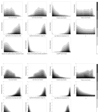
Figure 3. Emergent patterns: observed burnt area and predicted probabilities plotted against each predictor variable in turn. We show the
density of the data superimposed onto logarithmic density using 50 bins.
obscured.) We focus on comparing the forms of the relation-ships. The key point is that they are rarely the same as the underlying partial relationships as fitted by the GLM, and yet they are successfully predicted post hoc by the GLM. For example, although the underlying relationship between burnt area and NPP is monotonically increasing, the emer-gent pattern is unimodal, with a peak at 380 g C m−2a−1. This unimodal pattern is nonetheless correctly predicted by the GLM (Fig. 3). Low NPP results in fuel limitation, and the initial increase in burnt area with NPP is a consequence of the removal of this limitation. The apparent decrease in
Bu rn t a re a f ra c ti o n Bu rn t a re a f ra c ti o n Bu rn t a re a f ra c ti o n Bu rn t a re a f ra c ti o n Pr e d ic te d b u rn t a re a Pr e d ic te d b u rn t a re a Pr e d ic te d b u rn t a re a Pr e d ic te d b u rn t a re a
Log-Population density (people/km2) Log-Population density (people/km2
) Log-Gross annual product (US$) Log-Gross annual product (US$)
Mean annual precipitation (mm) Mean annual precipitation (mm) Mean annual temperature (o
[image:9.612.98.498.63.211.2]C) Mean annual temperature (oC)
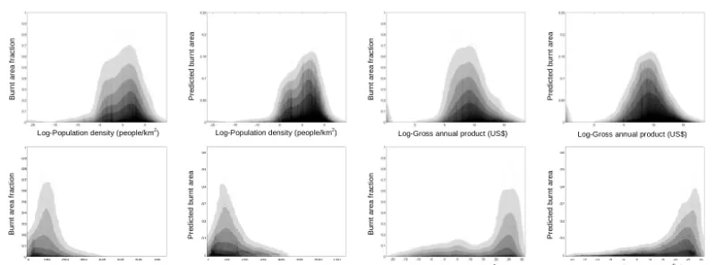
Figure 4. Emergent patterns: predicted probabilities against mean annual temperature (MAT), mean annual precipitation (MAP), ln
(popu-lation density) and ln (GDP per unit area). We show the density of the data superimposed onto logarithmic density using 50 bins.
A number of variables outside our set of predictors have been shown to correlate with burnt area (Fig. 4). Our GLM can also predict the emergent relationships with these vari-ables. Daniau et al. (2012), for example, from an analysis of remotely sensed burnt area and the charcoal palaeo record of biomass burning, showed that fire increases monotoni-cally with mean annual temperature (MAT). We predict the same steeply positive emergent response (Fig. 4), but also an extremely steep decline at the very highest temperatures, which are encountered only in exceptionally dry environ-ments where there is little or no fuel to burn. Van der Werf et al. (2008) showed a unimodal relationship between fire in the tropics and subtropics and mean annual precipitation (MAP), and this response has been replicated in a process-based model (Prentice et al., 2011). Our GLM also predicts a uni-modal relationship between burnt area and MAP. This re-lationship emerges because fuel availability (through NPP) is strongly controlled by MAP, while the fuel is too wet to burn in climates with high MAP (van der Werf et al., 2008; Archibald et al., 2009).
A number of analytical studies of both regional and global data sets have shown a unimodal relationship between burnt area and human population density, when log-transformed to emphasise the form of the relationship at very low popula-tion densities (Archibald et al., 2009; Aldersley et al., 2011; Bistinas et al., 2013). We also predict this unimodal response, even though the underlying fitted relationship is monotoni-cally decreasing. The emergent relationship is therefore an accurate representation of how population affects fire fre-quency with other factors held constant. It emerges simply because regions with very low NPP generally support low population densities. Similarly, the emergent unimodal re-lationship between fire and gross domestic product (GDP), shown by Aldersley et al. (2011), is an artefact caused by the automatic correlation of GDP (expressed per unit area) with population density.
4 Discussion
We have shown that NPP is a key control on burnt area, not surprisingly as NPP determines the amount of fuel avail-able to burn. The importance of NPP has been one of the most consistent results emerging from previous studies (e.g. Krawchuk et al., 2009; Aldersley et al., 2011; Moritz et al., 2012). Fire is limited in regions of low NPP because of lack of fuel or the discontinuous nature of the fuel. Regions of high NPP however are always associated with high precipi-tation. As a result, burnt area declines at high NPP, but high NPP is not the cause of this decline. We can simulate this pattern, because our GLM includes the relevant climatic pre-dictors as well as NPP.
Given the importance of NPP, it might be expected that other aspects of vegetation – influencing the flammability of fuel – would influence burnt area. There is indeed a strong relationship between burnt area and grass/shrub cover. This is probably due to the predominance of fast-drying fine fuels in grasslands and shrublands, compared to the coarser woody fuels that comprise much of the litter in forests.
We have shown that burnt area declines with soil moisture, while increasing with all three components of the Nesterov index, representing time since rain, maximum temperature, and vapour pressure deficit, respectively. Many other fire in-dices include similar components (see Alexander et al., 1996; Noble et al., 1980; Hardy and Hardy, 2007). Our analysis implies that each one of these components is independently necessary for a realistic prediction of burnt area. However, the strong relationship withαindicates that these three are not sufficient; soil moisture, with a much longer “memory” than litter moisture, is of major importance as well. We sug-gest that this is because soil moisture (a) controls the mois-ture content of live fuels, and (b) influences the rate at which foliage in highly seasonal climates (e.g. grass leaves in tropi-cal savannas) is “cured”, i.e. transitioning from living, turgid leaves into highly flammable fine litter.
Our analysis confirms the importance of human agency in influencing burnt area – but not always in the ways com-monly envisaged. Cropland area, as expected, has a neg-ative relationship with burnt area. The steep negneg-ative re-lationship between croplands and fire provides support for the idea that landscape fragmentation associated with in-tensive agriculture limits burnt area (see e.g. Marlon et al., 2008; Archibald et al., 2013) by reducing fuel connectivity. Grazing-land area however has a positive relationship with burnt area, suggesting that the effect of grazing in reducing fuel load (implemented as an effect reducing fire in some models; e.g. Krinner et al., 2005) is outweighed by other fac-tors, which may include the increase in fine fuel promoted by forest conversion, and continuing rangeland management. Many rangelands are in areas that would otherwise be domi-nated by natural grasslands, so the amount of grazed land is unlikely to reduce landscape connectivity.
Human population density shows a strong and consis-tently negative relationship with burnt area, which is signif-icant despite the separate inclusion of cropland and
grazing-land area. The role of people in suppressing fire has been identified through previous analyses of observations on biomass burning on recent, historic and palaeo timescales (e.g. Krawchuk and Moritz, 2009; Carcaillet et al., 2009; Marlon et al., 2008), and is attributed in part to direct in-tervention, but largely to a result of landscape fragmentation and fuel reduction. Given the independent relationships with cropland and grazing area – terms which already incorporate some aspects of landscape fragmentation or fuel removal – our analyses indicate that other human activities are also im-portant in suppressing fires and thus limiting the area and biomass burnt. Possible mechanisms include the removal of wood for heating and cooking, roads and clearings creating barriers to fire spread, and fragmentation through urbanisa-tion. It is likely that the mechanisms are different at different levels of population density and in different regions (Bistinas et al., 2013; Knorr et al., 2014).
Many modelling groups have included some form of fire suppression by humans. The most common approach is to mask fire in cropland (e.g. Thonicke et al., 2010; Prentice et al., 2011; Kelley et al., 2014) or as a universal (e.g. Pe-chony and Shindell, 2009; Kloster et al., 2010; Li et al., 2012) or spatially variable (tuned) function of population density (Thonicke et al., 2010), or by reducing fuel loads in grazing areas (Krinner et al., 2005). Clearly, given the independent relationships with cropland area and human population den-sity, the reliance on crop masking is insufficient. The reduc-tion of fuel loads in grazing land is not supported by the pos-itive relationship between burnt area and grazing-land area. Suppression of fire as a function of population density is con-sistent with our findings, but should be applied even at low population densities. Thus, models incorporating algorithms that increase fire as a result of increasing population density and then subsequently allow for fire suppression at higher population densities are not mechanistically consistent with the observed relationships.
It is implausible that burnt area decreases as lightning ig-nitions increase, and our second analysis showed that the ini-tially fitted negative relationship of lightning to burnt area must be an artefact of other, yet-to-be-determined processes with a strong seasonal cycle – such as day-length effects on phenology in seasonal climates. Pre-emptive burning before weather conditions become most suitable for large wildfires (Le Page et al., 2010) may also be a factor in synchronising the timing of fires with the seasonal cycle, and would also be expected to contribute to the human-induced reduction in burnt area.
Our results question some widely held assumptions about what controls fire. These assumptions underpin both the se-lection of variables included in statistical models, and the treatment of fire in DGVMs:
fragmentation on fire spread, implied by the strength of the negative influence of cropland on burnt area. 2. DGVMs have assumed that burnt area increases in
pro-portion to ignitions by lightning and/or people. Light-ning has no significant effect, indicating that the number of lightning strikes is not a limiting factor on biomass burning, and specifically on burnt area. These conclu-sions support the suggestion of Knorr et al. (2014) that ignition sources rarely or never limit fire frequency. Al-though there may be considerable spatial and temporal variability in the number of lightning-induced fire starts, as well as regional differences in the relative importance of natural and anthropogenic fire starts, this variability is ultimately unimportant in determining burnt area. Im-posing a strong and explicit link between the number of fire starts and burnt area in a model will lead to erro-neous predictions. We have shown that an apparent in-crease in burnt area with increasing population density at low population densities is an artifact of the relation-ship between NPP and population density. Given that models already incorporate the effect of fuel limitation on burning, including a second constraint through pop-ulation density will lead to erroneous predictions. The strong negative relationship between population density and burnt area, which is independent of constraints on burnt area due to land use, implies that it is important to include fire suppression in a modelling framework. In addition to fire-management activities, fire suppression could be a result of non-agricultural landscape fragmen-tation, the creation of artificial barriers to fire spread, and the removal of fuel for domestic use. Given that the causes of fire suppression are likely to vary spatially and with population density and cultural factors, further analyses of this phenomenon would be worthwhile. 3. Unimodal relationships between burnt area and climate
variables, which have been used in some statistical mod-els, have no mechanistic basis, and are therefore likely to mispredict burnt area when global conditions change, for example due to decoupled changes in temperature and precipitation, or due to increasing CO2
concentra-tions.
The increasing availability and quality control of global data sets on fire provides an opportunity for further data-driven analyses of fire to inform model development. We anticipate that this will lead to major changes in the way fire is repre-sented in models.
5 Summary and conclusions
Appendix A: Cross-correlation matrix and fitting criterion
For the correlation matrix, see Table A1.
[image:12.612.51.545.199.317.2]In order to assess the relative quality of our statistical model, we use the Akaike information criterion (AIC) as AIC=2N−2 ln(L),
Table A1. Cross-correlation matrix of all variables used for model fitting. We show Spearman’sρcoefficients.
1 2 3 4 5 6 7 8 9 10 11 12
1. Burnt area fraction 1.0000 0.0095 0.0344 −0.0166 0.0774 0.0973 0.0925 0.0681 0.0045 0.0289 −0.0124 −0.0911
2. Tree cover fraction 0.0095 1.0000 −0.5062 −0.1550 −0.3039 −0.3470 0.0065 0.1153 0.2442 0.4986 −0.0818 0.3408
3. Non-tree cover fraction 0.0344 −0.5062 1.0000 0.4157 0.3846 0.1926 0.1939 0.0574 −0.0041 −0.0945 0.1755 −0.1098
4. Cropland area fraction −0.0166 −0.1550 0.4157 1.0000 0.0658 0.1022 0.0806 0.1944 0.1595 0.1317 0.4903 0.0673
5. Grazing-land area fraction 0.0774 −0.3039 0.3846 0.0658 1.0000 0.3205 0.4195 0.2742 0.1562 −0.3917 −0.0077 −0.2445
6. Log-fraction dry days per month 0.0973 −0.3470 0.1926 0.1022 0.3205 1.0000 0.4971 0.0905 −0.1419 −0.4737 0.0665 −0.3145
7. Log-diurnal temperature range 0.0925 0.0065 0.1939 0.0806 0.4195 0.4971 1.0000 0.3665 0.2282 −0.2327 −0.0090 −0.1650
8. Log-maximum temperature 0.0680 0.1153 0.0574 0.1944 0.2742 0.0905 0.3665 1.0000 0.4905 0.0740 0.2814 0.1536
9.α −0.0911 0.2442 −0.0041 0.1595 0.1562 −0.1419 0.2282 0.4905 1.0000 0.2520 0.2203 0.1719
10. Square-root lightning flashes 0.0045 0.4986 −0.0945 0.1317 −0.3917 −0.4737 −0.2327 0.0740 0.2520 1.0000 0.1585 0.4911
11. Square-root population density −0.0124 −0.0818 0.1755 0.4903 −0.0077 0.0665 −0.0090 0.2814 0.2203 0.1585 1.0000 0.0722
12. Log NPP 0.0289 0.3408 −0.1098 0.0673 −0.2445 −0.3145 −0.1650 0.1536 0.1719 0.4911 0.0722 1.0000
whereN is the number of parameters used in the model and
Acknowledgements. This study was funded by Marie Curie
research training network GREENCYCLES II, contract number MRTN-CT-2004 (http://www.greencycles.org). The paper is a contribution to the AXA Chair Programme on Biosphere and Climate Impacts and the Imperial College initiative on Grand Challenges in Ecosystems and the Environment.
Edited by: P. Cox
References
Aldersley, A., Murray, S. J., and Cornell, S. E.: Global and regional analysis of climate and human drivers of wildfire, Sci. Total En-viron., 409:3472-81, doi:10.1016/j.scitotenv.2011.05.032, 2011. Alexander, M. E., Stocks, B. J., and Lawson, B. D.: The Canadian Forest Fire Danger Rating System, Initial Attack 1996 (Spring): 6–9, 1996.
Amatulli, G., Camia, A., and San-Miguel-Ayanz, J.: Estimat-ing future burned areas under changEstimat-ing climate in the EU-Mediterranean countries, Sci. Total Environ., 450–451, 209–22. doi:10.1016/j.scitotenv.2013.02.014, 2013.
Archibald, S., Roy, D. P., van Wilgen, B., and Scholes, R. J.: What limits fire? An examination of drivers of burnt area in Southern Africa, Glob. Chang Biol., 15, 613–630, 2009.
Archibald, S., Lehmann, C. E. R. L., Gomez-Dans, J. L., and Brad-stock, R. S.: Defining pyromes and global syndromes of fire regimes, PNAS, 110, 6442–6447, 2013.
Arneth, A., Harrison, S. P., Zaehle, S., Tsigaridis, K., Menon, S., Bartlein, P. J., Feichter, H., Korhola, A., Kulmala, M., O’Donnell, D., Schurgers, G., Sorvari, S., Vesala, T., and Zaehle, S.: Terrestrial biogeochemical feedbacks in the climate system, Nat. Geosci., 3, 525–532. doi:10.1038/ngeo905, 2010.
Balzter, H., Gerard, F., Weedon, G., Grey, W., Combal, B., Bartholome, E., Bartalev, S., and Los, S: Coupling of vegeta-tion growing season anomalies with hemispheric and regional scale climate patterns in Central and East Siberia, J. Climate, 20, 3713–3729, 2007.
Bartlein, P., Hostetler, S. W., Shafer, S. L., Holman, J. O., and Solomon, A. M.: Temporal and spatial structure in a daily wild-fire start dataset from the western United States (1986–96), Int J Wildland Fire, 17, 8–17, 2008.
Bistinas, I., Oom, D., Sá, A. C. L., Harrison, S. P., Prentice, I. C., and Pereira, J. M. C.: Relationships between Human Population Density and Burned Area at Continental and Global Scales, PLoS ONE, 8, e81188, doi:10.1371/journal.pone.0081188, 2013. Bond, W. J. and Wilgen, B.: Fire and plants, Chapman and Hall,
London, UK, 1996.
Bowman, D. M. J. S., Balch, J. K., Artaxo, P., Bond, W. J., Cochrane, M. A., and D’Antonia, C. M.: Fire in the earth sys-tem, Science, 324, 481–484, 2009.
Brovkin, V., van Bodegom, P. M., Kleinen, T., Wirth, C., Cornwell, W. K., Cornelissen, J. H. C., and Kattge, J.: Plant-driven variation in decomposition rates improves projections of global litter stock distribution, Biogeosciences, 9, 565–576, doi:10.5194/bg-9-565-2012, 2012.
Carcaillet, C., Ali, A. A., Blarquez, O., Genries, A., Mourier, B., and Bremond, L.: Spatial variability of fire history in subalpine forests: From natural to cultural regimes, Ecoscience, 16, 1–12, 2009.
Chang, J. F., Viovy, N., Vuichard, N., Ciais, P., Wang, T., Cozic, A., Lardy, R., Graux, A.-I., Klumpp, K., Martin, R., and Sous-sana, J.-F.: Incorporating grassland management in ORCHIDEE: model description and evaluation at 11 eddy-covariance sites in Europe, Geosci. Model Dev., 6, 2165–2181, doi:10.5194/gmd-6-2165-2013, 2013.
Cecil, D. J., Buechler, D. E., and Blakeslee, R. J.: Gridded lightning climatology from TRMM-LIS and OTD. Dataset description, At-mos. Res., 135–136, 404–414, 2014.
Center for International Earth Science Information Network (CIESIN), Columbia University, Centro Internacional de Agri-cultura Tropical (CIAT): Gridded population of the World Ver-sion 3 (GPWv3): population density grids, Socioeconomic Data and Applications Center (SEDAC), Columbia University, Pal-isades, 2005.
Cohen, J., Cohen, P., West, S. G, and Aiken, L. S.: Applied mul-tiple regression/correlation analysis for the behavioral sciences, Mhwah, NJ: Lawrence Erlbaum Associates, 3rd Edition, 2003. Dai, A., Trenberth, K. E., and Karl, T. R.: Effects of clouds, soil
moisture, precipitation and water vapor on diurnal temperature range, J. Clim., 12, 2451–2473, 1999.
Daniau, A.-L., Bartlein, P. J., Harrison, S. P., Prentice, I. C., Brewer, S., Friedlingstein, P., Harrison-Prentice, T. I., Inoue, J., Izumi, K., Marlon, J. R., Mooney, S., Power, M. J., Stevenson, J., Tinner, W., Andriˇc, M., Atanassova, J., Behling, H., Black, M., Blar-quez, O., Brown, K. J., Carcaillet, C., Colhoun, E. A., Colom-baroli, D., Davis, B. A. S., D’Costa, D., Dodson, J., Dupont, L., Eshetu, Z., Gavin, D. G., Genries, A., Haberle, S., Hallett, D. J., Hope, G., Horn, S. P., Kassa, T. G., Katamura, F., Kennedy, L. M., Kershaw, P., Krivonogov, S., Long, C., Magri, D., Mari-nova, E., McKenzie, G. M., Moreno, P. I., Moss, P., Neumann, F. H., Norström, E., Paitre, C., Rius, D., Roberts, N., Robin-son, G. S., Sasaki, N., Scott, L., Takahara, H., Terwilliger, V., Thevenon, F., Turner, R., Valsecchi, V. G., Vannière, B., Walsh, M., Williams, N. and Zhang, Y. : Predictability of biomass burn-ing in response to climate changes, Global Biogeochem. Cy., 26: doi:10.1029/2011GB004249, 2012.
DeFries, R. and Hansen, M. C.: ISLSCP II Continuous Fields of Vegetation Cover, 1992–1993, in: ISLSCP Initiative II Collec-tion, Dataset, edited by: Hall, F. G., Collatz, G., Meeson, B., Los, S., Brown De Colstoun, E., and Landis, D., Oak Ridge, Ten-nessee, USA, available at: http://daac.ornl.gov/ from Oak Ridge National Laboratory Distributed Active Archive Center (last ac-cess: 20 July 2013), 2009.
DiMiceli, C. M., Carroll, M. L., Sohlberg, R. A., Huang, C., Hansen, M. C., and Townshend, J. R. G.: Annual Global Au-tomated MODIS Vegetation Continuous Fields (MOD44B) at 250 m Spatial Resolution for Data Years Beginning Day 65, 2000–2010, Collection 5 Percent Tree Cover. University of Maryland, College Park, MD, USA, 2011.
European Environmental Agency: Climate change, impacts and vul-nerability in Europe 2012: An indicator-based report, European Environmental Agency, 300 pp., 2012.
Fernandes, P. M., Davies, G. M., Ascoli, D., Fernández, C., Mor-eira, F., Rigolot, E., Stoof, C. R., Vega, J. A., and Molina, D.: Prescribed burning in southern Europe: developing fire manage-ment in a dynamic landscape, Front. Ecol. Environ., 11, e4–e14, doi:10.1890/120298, 2013.
Gallego-Sala, A. V., Clark, J. M., House, J. I., Orr, H. G., Prentice, I. P., Smith, P., Farewell, T., and Chapman, S. J.: Bioclimatic envelope model of climate change impacts on blanket peatland distribution in Great Britain, Clim. Res. 45, 151–162, 2010. Giglio, L, Csiszar, I., and Justice, C. O.: Global distribution
and seasonality of active fires as observed with the Terra and Aqua MODIS sensors, J. Geophys. Res.-Biogeo., 111, G02016, doi:10.1029/2005JG000142, 2006.
Giglio, L., Randerson, J. T., van der Werf, G. R., Kasibhatla, P. S., Collatz, G. J., Morton, D. C., and DeFries, R. S.: Assess-ing variability and long-term trends in burned area by mergAssess-ing multiple satellite fire products, Biogeosciences, 7, 1171–1186, doi:10.5194/bg-7-1171-2010, 2010.
Giglio, L., Randerson, J. T., and van der Werf, G. R.: Analy-sis of daily, monthly, and annual burned area using the fourth-generation global emissions database (GFED4), J. Geophys. Res.-Biogeo., 118, 317–328, 2013.
Guyette, R. P., Muzika, R. M., and Dey, D. C.: Dynamics of an anthropogenic fire regime, Ecosystems, 5, 472–486, doi:10.1007/s10021-002-0115-7, 2002.
Hardy, C. C. and Hardy, C. E.: Fire danger rating in the United States of America: an evolution since 1916, International Journal of Wildland Fire, 16, 217–231, 2007.
Harrison, S. P., Marlon, J., and Bartlein, P. J.: Fire in the Earth Sys-tem, in: Changing Climates, Earth Systems and Society, edited by: Dodson, J., Springer-Verlag, 21–48, 2010.
Kelley, D. I., Prentice, I. C., Harrison, S. P., Wang, H., Simard, M., Fisher, J. B., and Willis, K. O.: A comprehensive benchmarking system for evaluating global vegetation models, Biogeosciences, 10, 3313–3340, doi:10.5194/bg-10-3313-2013, 2013.
Kelley, D. I., Harrison, S. P., and Prentice, I. C.: Improved simula-tion of fire-vegetasimula-tion interacsimula-tions in the Land surface Processes and eXchanges dynamic global vegetation model (LPX-Mv1), Geosci. Model Dev. Discuss., 7, 931–1000, doi:10.5194/gmdd-7-931-2014, 2014.
Klein Goldewijk, K., Beusen, A., Van Drecht, G., and De Vos, M.: The HYDE 3.1 spatially explicit database of human-induced global land-use change over the past 12 000 years, Global Ecol. Biogeogr., 20, 73–86, 2011.
Kloster, S., Mahowald, N. M., Randerson, J. T., Thornton, P. E., Hoffman, F. M., Levis, S., Lawrence, P. J., Feddema, J. J., Ole-son, K. W., and Lawrence, D. M.: Fire dynamics during the 20th century simulated by the Community Land Model, Biogeo-sciences, 7, 1877–1902, doi:10.5194/bg-7-1877-2010, 2010. Knorr, W. and Heimann, M.: Impact of drought stress and other
fac-tors on seasonal land biosphere CO2exchange studied through
an atmospheric tracer transport model, Tellus B, 47, 471–489, 1995.
Knorr, W., Kaminski, T., Arneth, A., and Weber, U.: Impact of hu-man population density on fire frequency at the global scale, Biogeosciences, 11, 1085–1102, doi:10.5194/bg-11-1085-2014, 2014.
Krawchuk, M. A. and Moritz, M. A.: Fire regimes of China: Infer-ence from statistical comparison with the United States, Global Ecol. Biogeogr., 18, 626–639, 2009.
Krawchuk, M. A., Moritz, M. A., Parisien, M.-A., Van Dorn, J., and Hayhoe, K.: Global pyrogeography: The current and future distribution of wildfire, PLoS ONE, 4, e5102, doi:10.1371/journal.pone.0005102, 2009.
Krinner, G., Viovy, N., Noblet-Ducoudré, N., Ogé, J., Polcher, J., and Friedlingstein, P.: A dynamic global vegetation model for studies of the coupled atmosphere-biosphere system, Global Bio-geochem. Cy., 1, GB1015, doi:10.1029/2003GB002199, 2005. Larsen, W. A. and McCleary, S. J.: The use of partial residual plots
in regression analysis, Technometrics, 14, No. 3 (August 1972), 781–790, 1972.
Lavorel, S., Flannigan, M., Lambin, E., and Scholes, M.: Vulner-ability of land systems to fire: Interactions among humans, cli-mate, the atmosphere, and ecosystems, Mitig Adapt Strat Glob Change 12, 33–53, 2007.
Lehsten, V., Harmand, P., Palumbo, I., and Arneth, A.: Mod-elling burned area in Africa, Biogeosciences, 7, 3199–3214, doi:10.5194/bg-7-3199-2010, 2010.
Li, F., Zeng, X. D., and Levis, S.: A process-based fire parameteriza-tion of intermediate complexity in a Dynamic Global Vegetaparameteriza-tion Model, Biogeosciences, 9, 2761–2780, doi:10.5194/bg-9-2761-2012, 2012.
Marlon, J., Bartlein. P. J., Carcaillet, C., Gavin, D. G., Harrison, S. P., Higuera, P. E., Joos, F., Power, M. J., and Prentice, I. C.: Climate and human influences on global biomass burning over the past two millennia, Nat. Geosci., 1, 697–701, 2008. Maxwell, S. E.: Sample size and multiple regression analysis,
Psychol. Methods, 5, 434–458, doi:10.1037/1082-989X.5.4.434, 2000.
McFadden, D.: Conditional logit analysis of qualitative choice be-havior, in: Frontiers in Econometrics, edited by: Zarembka, P. , Academic Press, 105–142 1974.
Moritz, M. A., Parisien, M.-A., Batllori, E., Krawchuk, M. A., Van Dorn, J., Ganz, D. J. and Hayhoe, K.: Climatic changes and disruptions to global fire activity, Ecosphere, 3, 49, doi:10.1890/ES11-00345.1, 2012.
Nesterov, V. G.: Flammability of the Forest and Methods for Its De-termination, (Gorimost lesa i metodi eio opredelenia), Goslesbu-mizdat, USSR State Ind. Press, Moscow, 1949 (in Russian). Noble I. R., Bary G. A. A., and Gill A. M.: McArthur’s fire danger
meters expressed as equations, Australian Journal of Ecology, 5, 201–203, 1980.
Page Le, Y., Oom, D., Silva, J. M. N., Jonsson, P., and Pereira, J. M. C. : Seasonality of vegetation fires as modified by human action: Observing the deviation from eco-climatic fire regimes, Global Ecol. Biogeogr., 19, 575–588, 2010.
Papke, L. E. and Wooldridge, J.: Econometric Methods for Frac-tional Response Variables with an Application to 401(k) Plan Participation Rates, J. Appl. Econom., 11, 619–632, 1996. Parisien, M. A. and Moritz, M. A.: Environmental controls on the
distribution of wildfire at multiple spatial scales, Ecol. Monogr., 79, 127–154, 2009.
Pechony, O. and Shindell, D. T.: Fire parameterization on a global scale, J. Geophys. Res., 114, 1–10, 2009.
North American boreal forest: implications for fire weather fore-casting, Atmos. Chem. Phys., 10, 6873–6888, doi:10.5194/acp-10-6873-2010, 2010.
Pfeiffer, M., Spessa, A., and Kaplan, J. O.: A model for global biomass burning in preindustrial time: LPJ-LMfire (v1.0), Geosci. Model Dev., 6, 643–685, doi:10.5194/gmd-6-643-2013, 2013.
Prentice, I. C., Sykes, M. T., and Cramer, W.: A simulation model for the transient effects of climate change on forest landscapes, Ecol. Model., 65, 51–70, 1993.
Prentice, I. C., Kelley, D. I., Foster, P. N., Friedlingstein, P., Har-rison, S. P., and Bartlein, P. J.: Modeling fire and the terres-trial carbon balance, Global Biogeochem. Cy., 25, GB3005, doi:10.1029/2010GB003906, 2011.
Pyne, S. J.: Fire: Nature and Culture, Reaktion Books, London, 224 pp., 2012.
Rothermel, R. C.: A mathematical model for predicting fire spread in wildland fuels, Gen. Tech. Rep. INT-115, US Dep. of Agric., For. Serv., Intermt. For. and Range Exp. Stn., Ogden, Utah, 1972. Running, S. W.: Is global warming causing more, larger wildfires?,
Science 313, 927–928, 2006.
Sanderson, E., Jaiteh, M., Levy, M., Redford, K., Wannebo, V., and Woolmer, G.: The human footprint and the last of the wild, Bio-science, 52, 891–904, 2002.
Scholze, M., Knorr, W., Arnell, N. W., and Prentice, I. C.: A climate change risk analysis for world ecosystems, P. Natl. Acad. Sci. USA, 103, 13116–13120, doi:10.1073/pnas.0601816103, 2006. Sheridan, P.: Review of techniques and research for gust forecasting
parameterization, Forecasting Research Technical Report 570, UK Met Office, Exeter, 2011.
Syphard, A. D., Radeloff, V. C., Hawbaker, T. J., and Stewart, S. I.: Conservation threats due to human-caused increases in fire frequency in Mediterranean-climate ecosystems, Conserv. Biol., 23, 758–769, 2009.
Thonicke, K., Spessa, A., Prentice, I. C., Harrison, S. P., Dong, L., and Carmona-Moreno, C.: The influence of vegetation, fire spread and fire behaviour on biomass burning and trace gas emis-sions: results from a process-based model, Biogeosciences, 7, 1991–2011, doi:10.5194/bg-7-1991-2010, 2010.
Wang, H., Prentice, I. C., and Ni, J.: Data-based modelling and en-vironmental sensitivity of vegetation in China, Biogeosciences, 10, 5817–5830, doi:10.5194/bg-10-5817-2013, 2013.
van der Werf, G. R., Randerson, J. T., Giglio L., Gobron, N., and Dolman A. J.: Climate controls on the variability of fires in the tropics and subtropics, Global Biogeochem. Cy., 22, GB3028, doi:10.1029/2007GB003122, 2008.
van der Werf, G. R., Randerson, J. T., Giglio, L., Collatz, G. J., Mu, M., Kasibhatla, P. S., Morton, D. C., DeFries, R. S., Jin, Y., and van Leeuwen, T. T.: Global fire emissions and the contribution of deforestation, savanna, forest, agricultural, and peat fires (1997– 2009), Atmos. Chem. Phys., 10, 11707–11735, doi:10.5194/acp-10-11707-2010, 2010.
Westerling, A. L., Hidalgo, H. G., Cayan, D. R., and Swetnam, T. W.: Warming and earlier Spring increases Western U.S. forest wildfire activity, Science, 313, 940–943, 2006.