(a)t 1 sec? (b) t5 sec? SOLUTION Solve Analytically (a) The position at t1 is the initial positions0 plus the displacement (the

Chapter

7

_{Applications of}

Definite Integrals

T

he art of pottery developed independently

in many ancient civilizations and still exists in

modern times. The desired shape of the side

of a pottery vase can be described by:

y

5.0

2 sin (

x

/4) (0

x

8

p

)

where

x

is the height and

y

is the radius at

height

x

(in inches).

A base for the vase is preformed and placed on a

potter’s wheel. How much clay should be added to

the base to form this vase if the inside radius is

al-ways 1 inch less than the outside radius? Section 7.3

contains the needed mathematics.

Chapter 7 Overview

By this point it should be apparent that finding the limits of Riemann sums is not just an

intellectual exercise; it is a natural way to calculate mathematical or physical quantities

that appear to be irregular when viewed as a whole, but which can be fragmented into

reg-ular pieces. We calculate values for the regreg-ular pieces using known formulas, then sum

them to find a value for the irregular whole. This approach to problem solving was around

for thousands of years before calculus came along, but it was tedious work and the more

accurate you wanted to be the more tedious it became.

With calculus it became possible to get

exact

answers for these problems with almost

no effort, because in the limit these sums became definite integrals and definite integrals

could be evaluated with antiderivatives. With calculus, the challenge became one of fitting

an integrable function to the situation at hand (the “modeling” step) and then finding an

antiderivative for it.

Today we can finesse the antidifferentiation step (occasionally an insurmountable

hur-dle for our predecessors) with programs like NINT, but the modeling step is no less

cru-cial. Ironically, it is the modeling step that is thousands of years old. Before either calculus

or technology can be of assistance, we must still break down the irregular whole into

regu-lar parts and set up a function to be integrated. We have already seen how the process

works with area, volume, and average value, for example. Now we will focus more closely

on the underlying modeling step: how to set up the function to be integrated.

Integral As Net Change

Linear Motion Revisited

In many applications, the integral is viewed as net change over time. The classic example

of this kind is distance traveled, a problem we discussed in Chapter 5.

EXAMPLE 1

Interpreting a Velocity Function

Figure 7.1 shows the velocity

d

_d

s

_t

v

(

t

)

t

t

8

1

of a particle moving along a horizontal

s

-axis for 0

t

5. Describe the motion.

SOLUTION

Solve Graphically

The graph of

v

(Figure 7.1) starts with

v

0

8, which we

in-terpret as saying that the particle has an initial velocity of 8 cm

sec to the left. It slows to a

halt at about

t

1.25 sec, after which it moves to the right

v

0

with increasing speed,

reaching a velocity of

v

5

24.8 cm

sec at the end.

EXAMPLE 2

Finding Position from Displacement

Suppose the initial position of the particle in Example 1 is

s

0

9. What is the

parti-cle’s position at

(a)

t

1 sec?

(b)

t

5 sec?

SOLUTION

Solve Analytically

(a)

The position at

t

1 is the initial position

s

0

plus the displacement (the

amount,

Δ

s

, that the position changed from

t

0 to

t

1). When velocity is

7.1

What you’ll learn about

• Linear Motion Revisited

• General Strategy

• Consumption Over Time

• Net Change from Data

• Work

. . . and why

The integral is a tool that can be

used to calculate net change and

total accumulation.

continued

constant during a motion, we can find the displacement (change in position) with the

formula

Displacement

rate of change

time.

But in our case the velocity varies, so we resort instead to partitioning the time interval

0, 1

into subintervals of length

Δ

t

so short that the velocity is effectively constant on

each subinterval. If

t

is any time in the

k

th subinterval, the particle’s velocity throughout

that interval will be close to

v

t

. The change in the particle’s position during the brief

time this constant velocity applies is

v

t

Δ

t.

If

v

t

is negative, the displacement is negative and the particle will move left. If

v

t

is positive, the particle will move right. The sum

v

t

Δ

t

of all these small position changes approximates the displacement for the time interval

0, 1

.

The sum

v

t

Δ

t

is a Riemann sum for the continuous function

v

t

over

0, 1

. As

the norms of the partitions go to zero, the approximations improve and the sums

con-verge to the integral of

v

over

0, 1

, giving

Displacement

1

0

v

t

dt

1

0

(

t

t

8

1

)

dt

[

t

₃

_t

8

₁

]

1

0

1

3

8

2

8

1

3

1

.

During the first second of motion, the particle moves 11

3 cm to the left. It starts at

s

0

9, so its position at

t

1 is

New position

initial position

displacement

9

1

3

1

1

3

6

.

(b)

If we model the displacement from

t

0 to

t

5 in the same way, we arrive at

Displacement

5

0

v

t

dt

[

t

3

3

t

8

1

]

5

0

35.

The motion has the net effect of displacing the particle 35 cm to the right of its starting

point. The particle’s final position is

Final position

initial position

displacement

s

0

35

9

35

44.

Support Graphically

The position of the particle at any time

t

is given by

s

t

0

[

u

u

8

1

]

du

9,

because

s

t

v

t

and

s

0

9. Figure 7.2 shows the graph of

s

t

given by the

parametrization

x

t

NINT

v

u

,

u

, 0,

t

9,

y

t

t

,

0

t

5.

Reminder from Section 3.4

A change in position is a displacement. If s(t) is a body’s position at time t, the displacement over the time interval from tto tΔtiss(tΔt)s(t). The displacement may be positive, negative, or zero, depending on the motion.

(a)

Figure 7.2a supports that the position of the particle at

t

1 is 16

3.

(b)

Figure 7.2b shows the position of the particle is 44 at

t

5. Therefore, the

dis-placement is 44

9

35.

The reason for our method in Example 2 was to illustrate the

modeling step

that will

be used throughout this chapter. We can also solve Example 2 using the techniques of

Chapter 6 as shown in Exploration 1.

Revisiting Example 2

The velocity of a particle moving along a horizontal

s

-axis for 0

t

5 is

d

_d

s

_t

t

t

8

1

.

1.

Use the indefinite integral of

ds

dt

to find the solution of the initial value

problem

d

_d

s

_t

t

t

8

1

,

s

0

9.

2.

Determine the position of the particle at

t

1. Compare your answer with the

answer to Example 2a.

3.

Determine the position of the particle at

t

5. Compare your answer with the

answer to Example 2b.

EXPLORATION 1

We know now that the particle in Example 1 was at

s

0

9 at the beginning of the

motion and at

s

5

44 at the end. But it did not travel from 9 to 44 directly—it began its

trip by moving to the left ( Figure 7.2). How much distance did the particle actually travel?

We find out in Example 3.

EXAMPLE 3

Calculating Total Distance Traveled

Find the

total distance traveled

by the particle in Example 1.

SOLUTION

Solve Analytically

We partition the time interval as in Example 2 but record every

position shift as

positive

by taking absolute values. The Riemann sum approximating

total distance traveled is

v

t

Δ

t,

and we are led to the integral

Total distance traveled

5

0

v

t

dt

5

0

t

t

8

1

dt

.

Evaluate Numerically

We have

NINT

(

t

t

8

1

,

t

, 0, 5

)

42.59.

Now try Exercise 1(c). [–10, 50] by [–2, 6]

(a) T = 1

X = 5.3333333 Y = 1

[–10, 50] by [–2, 6]

(b) T = 5

X = 44 Y = 5

Figure 7.2 Using TRACE and the

What we learn from Examples 2 and 3 is this: Integrating velocity gives displacement

(net area between the velocity curve and the time axis). Integrating the

absolute value

of

velocity gives total distance traveled (total area between the velocity curve and the time

axis).

General Strategy

The idea of fragmenting net effects into finite sums of easily estimated small changes is

not new. We used it in Section 5.1 to estimate cardiac output, volume, and air pollution.

What

is

new is that we can now identify many of these sums as Riemann sums and express

their limits as integrals. The advantages of doing so are twofold. First, we can evaluate one

of these integrals to get an accurate result in less time than it takes to crank out even the

crudest estimate from a finite sum. Second, the integral itself becomes a formula that

en-ables us to solve similar problems without having to repeat the modeling step.

The strategy that we began in Section 5.1 and have continued here is the following:

Strategy for Modeling with Integrals

1.

Approximate what you want to find as a Riemann sum

of values of a continuous

function multiplied by interval lengths. If

f

x

is the function and

a

,

b

the

inter-val, and you partition the interval into subintervals of length

Δ

x

, the

approximat-ing sums will have the form

f

c

Δ

x

with

c

a point in the

k

th subinterval.

2.

Write a definite integral,

here

f

x

dx

, to express the limit of these sums as

the norms of the partitions go to zero.

3.

Evaluate the integral

numerically or with an antiderivative.

EXAMPLE 4

Modeling the Effects of Acceleration

A car moving with initial velocity of 5 mph accelerates at the rate of

a

t

2.4

t

mph per second for 8 seconds.

(a)

How fast is the car going when the 8 seconds are up?

(b)

How far did the car travel during those 8 seconds?

SOLUTION

(a)

We first model the effect of the acceleration on the car’s velocity.

Step 1:

Approximate the net change in velocity as a Riemann sum.

When acceleration

is constant,

velocity change

acceleration

time applied.

To apply this formula, we partition

0, 8

into short subintervals of length

Δ

t.

On

each subinterval the acceleration is nearly constant, so if

t

is any point in the

k

th

subinterval, the change in velocity imparted by the acceleration in the subinterval is

approximately

a

t

Δ

t

mph.

p c

h sec

The net change in velocity for 0

t

8 is approximately

a

t

Δ

t

mph.

Step 2:

Write a definite integral.

The limit of these sums as the norms of the partitions

go to zero is

a

t

dt

.

Step 3:

Evaluate the integral.

Using an antiderivative, we have

Net velocity change

8

0

2.4

t dt

1.2

t

]

0

76.8 mph.

So, how fast is the car going when the 8 seconds are up? Its initial velocity is 5 mph and

the acceleration adds another 76.8 mph for a total of 81.8 mph.

(b)

There is nothing special about the upper limit 8 in the preceding calculation.

Apply-ing the acceleration for any length of time

t

adds

2.4

u du

mph

(b)

to the car’s velocity, giving

v

t

5

t

0

2.4

u du

5

1.2

t

_mph.

The distance traveled from

t

0 to

t

8 sec is

v

t

dt

8

0

5

1.2

t

_dt

[

5

t

0.4

t

]

0

244.8 mph

seconds.

Miles-per-hour second is not a distance unit that we normally work with! To convert to

miles we multiply by hours

second

1

3600, obtaining

244.8

36

1

00

0.068 mile.

m h i

sec se

h c mi

The car traveled 0.068 mi during the 8 seconds of acceleration.

Consumption Over Time

The integral is a natural tool to calculate net change and total accumulation of more

quan-tities than just distance and velocity. Integrals can be used to calculate growth, decay, and,

as in the next example, consumption. Whenever you want to find the cumulative effect of a

varying rate of change, integrate it.

EXAMPLE 5

Potato Consumption

From 1970 to 1980, the rate of potato consumption in a particular country was

C

t

2.2

1.1

_{millions of bushels per year, with}

_t

_{being years since the beginning of 1970.}

How many bushels were consumed from the beginning of 1972 to the end of 1973?

SOLUTION

We seek the cumulative effect of the consumption rate for 2

t

4.

Step 1:

Riemann sum.

We partition

2, 4

into subintervals of length

Δ

t

and let

t

be a time

in the

k

th subinterval. The amount consumed during this interval is approximately

C

t

Δ

t

million bushels.

The consumption for 2

t

4 is approximately

C

t

Δ

t

million bushels.

Step 2:

Definite integral.

The amount consumed from

t

2 to

t

4 is the limit of

these sums as the norms of the partitions go to zero.

C

t

dt

4

2

2.2

1.1

_dt

_{million bushels}

Step 3:

Evaluate.

Evaluating numerically, we obtain

NINT

2.2

1.1

_,

_t

_{, 2, 4}

_{7.066 million bushels.}

Now try Exercise 21.

Net Change from Data

Many real applications begin with data, not a fully modeled function. In the next example,

we are given data on the rate at which a pump operates in consecutive 5-minute intervals

and asked to find the total amount pumped.

EXAMPLE 6

Finding Gallons Pumped from Rate Data

A pump connected to a generator operates at a varying rate, depending on how much

power is being drawn from the generator to operate other machinery. The rate (gallons

per minute) at which the pump operates is recorded at 5-minute intervals for one hour

as shown in Table 7.1. How many gallons were pumped during that hour?

SOLUTION

Let

R

t

, 0

t

60, be the pumping rate as a continuous function of time for the hour.

We can partition the hour into short subintervals of length

Δ

t

on which the rate is nearly

constant and form the sum

R

t

Δ

t

as an approximation to the amount pumped

dur-ing the hour. This reveals the integral formula for the number of gallons pumped to be

Gallons pumped

60

0

R

t

dt

.

We have no formula for

R

in this instance, but the 13 equally spaced values in Table 7.1

enable us to estimate the integral with the Trapezoidal Rule:

0

R

t

dt

2

6

•

0

12

[

58

2

60

2

65

…

2

63

63

]

3582.5.

The total amount pumped during the hour is about 3580 gal.

Work

In everyday life,

work

means an activity that requires muscular or mental effort. In science,

the term refers specifically to a force acting on a body and the body’s subsequent

displace-ment. When a body moves a distance

d

along a straight line as a result of the action of a

force of constant magnitude

F

in the direction of motion, the

work

done by the force is

W

Fd.

The equation

W

Fd

is the

constant-force formula

for work.

The units of work are force

distance. In the metric system, the unit is the

newton-meter, which, for historical reasons, is called a joule (see margin note). In the U.S.

cus-tomary system, the most common unit of work is the

foot-pound.

Table 7.1 Pumping Rates

Time (min) Rate (gal

0 58

5 60

10 65

15 64

20 58

25 57

30 55

35 55

40 59

45 60

50 60

55 63

60 63

Joules

The joule, abbreviated J and pro-nounced “jewel,” is named after the English physicist James Prescott Joule (1818–1889). The defining equation is

1 joule (1 newton)(1 meter).

In symbols, 1 J 1 N • m.

Hooke’s Law

for springs says that the force it takes to stretch or compress a spring

x

units from its natural (unstressed) length is a constant times

x.

In symbols,

F

kx

,

where

k

, measured in force units per unit length, is a characteristic of the spring called the

force constant.

EXAMPLE 7

A Bit of Work

It takes a force of 10 N to stretch a spring 2 m beyond its natural length. How much work

is done in stretching the spring 4 m from its natural length?

SOLUTION

We let

F

x

represent the force in newtons required to stretch the spring

x

meters from

its natural length. By Hooke’s Law,

F

x

kx

for some constant

k.

We are told that

F

2

10

k

2,

so

k

5 N

m and

F

x

5

x

for this particular spring.

We construct an integral for the work done in applying

F

over the interval from

x

0

to

x

4.

Step 1:

Riemann sum.

We partition the interval into subintervals on each of which

F

is

so nearly constant that we can apply the constant-force formula for work. If

x

is any point in the

k

th subinterval, the value of

F

throughout the interval is

approximately

F

x

5

x

.

The work done by

F

across the interval is

approximately 5

x

Δ

x

, where

Δ

x

is the length of the interval. The sum

F

x

Δ

x

5

x

Δ

x

approximates the work done by

F

from

x

0 to

x

4.

Steps 2 and 3:

Integrate.

The limit of these sums as the norms of the partitions go to

zero is

F

x

dx

4

0

5

x dx

5

x

2

2

]

4

0

40 N

_m.

Now try Exercise 29.

We will revisit work in Section 7.5.

The force required to stretch the spring 2 m is 10 newtons.

Numerically, work is the area under the force graph.

Quick Review 7.1

(For help, go to Section 1.2.)

In Exercises 1–10, find all values of x(if any) at which the function changes sign on the given interval. Sketch a number line graph of the interval, and indicate the sign of the function on each subinterval.

Example: fxx2_{1 on 2, 3}

Changes sign at x 1.

1. sin 2x on 3, 2 Changes sign at p 2, 0,

p

2

2. x2_{3x2 on 2, 4 Changes sign at 1, 2} –2 –1

+ – +

1 3

f (x)

x

3. x2_{2x3 on 4, 2 Always positive} 4. 2x3_3x2_{1 on 2, 2 Changes sign at} 1

2

5. xcos 2x on 0, 4 Changes sign at p 4,

3 4

p ,5

4

p 6. xex _{on 0,}

∞

7.

x2

x

1

on 5, 30 Changes sign at 0

8. x

x

2

2

2 4

on 3, 3 Changes sign at 2, 2, 2, 2

9. sec1 1sin2_{x on}

∞

∞

3 1

p,2 1

p

In Exercises 1–8, the function v(t) is the velocity in m

(a)Determine when the particle is moving to the right, to the left, and stopped.

(b)Find the particle’s displacement for the given time interval. If

s(0)3, what is the particle’s final position? (c)Find the total distance traveled by the particle.

1. vt5 cost, 0t2p See page 389.

2. vt6 sin 3t, 0tp

3. vt499.8t, 0t10 See page 389.

4. vt6t2_{18t12, 0t2 See page 389.} 5. vt5 sin2_{tcost, 0t2p See page 389.} 6. vt 4t, 0t4 See page 389.

7. vtesint_{cost, 0t2p See page 389.}

8. vt

1

t t2

, 0t3 See page 389.

9. An automobile accelerates from rest at 13 tmph

(a)What is its velocity after 9 seconds? 63 mph

(b)How far does it travel in those 9 seconds? 344.52 feet

10.A particle travels with velocity

vtt2sint m

(a)What is the particle’s displacement? 1.44952 meters

(b)What is the total distance traveled? 1.91411 meters

11.Projectile Recall that the acceleration due to Earth’s gravity is 32 ft

(a)What is its velocity after 3 seconds? 6 ft/sec

(b)When does it hit the ground? 5.625 sec

(c)When it hits the ground, what is the net distance it has traveled? 0

(d)When it hits the ground, what is the total distance it has traveled? 253.125 feet

In Exercises 12–16, a particle moves along the x-axis (units in cm). Its initial position at t0 sec is x015. The figure shows the graph of the particle’s velocity vt. The numbers are the areasof the enclosed regions.

4

5

a b c

24

12.What is the particle’s displacement between t 0 and t c? 13.What is the total distance traveled by the particle in the same

time period? 33 cm

14.Give the positions of the particle at times a,b, and c.

15.Approximately where does the particle achieve its greatest positive acceleration on the interval 0,b? ta

16.Approximately where does the particle achieve its greatest positive acceleration on the interval 0,c? t c

In Exercises 17–20, the graph of the velocity of a particle moving on the x-axis is given. The particle starts at x 2 when t 0.

(a)Find where the particle is at the end of the trip.

(b)Find the total distance traveled by the particle.

17.

18.

19.

20.

21. U.S. Oil Consumption The rate of consumption of oil in the United States during the 1980s (in billions of barrels per year) is modeled by the function C 27.08•et25, where tis the number of years after January 1, 1980. Find the total consumption of oil in the United States from January 1, 1980 to January 1, 1990. 332.965 billion barrels

22.Home Electricity Use The rate at which your home consumes electricity is measured in kilowatts. If your home consumes electricity at the rate of 1 kilowatt for 1 hour, you will be charged

t (sec) v(m/sec)

0 1 3

2 3 4 5 6 7

– 3

8 9 10 t (sec) v(m/sec)

0 1 2

2 3 4 5 6 7

– 2 1

0

1 2 3 4

–1 v (m/sec)

t (sec) v (m/sec)

t (sec) 2

1 2 3 4 0

Section 7.1 Exercises

23 cm

a: 11 b: 16 c:8

(a)6 (b)4 meters

(a) 2 (b)4 meters

(a)5 (b)7 meters

for 1 “kilowatt-hour” of electricity. Suppose that the average consumption rate for a certain home is modeled by the function

Ct 3.9 2.4 sinpt

23.Population Density Population density measures the number of people per square mile inhabiting a given living area. Washerton’s population density, which decreases as you move away from the city center, can be approximated by the function 10,0002 r at a distance rmiles from the city center. (a) If the population density approaches zero at the edge of the city, what is the city’s radius? 2 miles

(b)A thin ring around the center of the city has thickness Δrand radius r.If you straighten it out, it suggests a rectangular strip. Approximately what is its area? 2prr

(c) Writing to Learn Explain why the population of the ring in part (b) is approximately

10,0002r2

p

(d) Estimate the total population of Washerton by setting up and evaluating a definite integral. 83,776

24.Oil Flow Oil flows through a cylindrical pipe of radius 3 inches, but friction from the pipe slows the flow toward the outer edge. The speed at which the oil flows at a distance r

inches from the center is 810 r2_{inches per second.} (a) In a plane cross section of the pipe, a thin ring with thickness Δrat a distance rinches from the center approximates a rectangular strip when you straighten it out. What is the area of the strip (and hence the approximate area of the ring)?

(b)Explain why we know that oil passes through this ring at approximately 810 r2_{2prΔr cubic inches per second.} (c)Set up and evaluate a definite integral that will give the rate (in cubic inches per second) at which oil is flowing through the pipe. 396pin3_{/sec or 1244.07 in}3_/sec

25.Group Activity Bagel Sales From 1995 to 2005, the

Konigsberg Bakery noticed a consistent increase in annual sales of its bagels. The annual sales (in thousands of bagels) are shown below.

Sales Year (thousands)

1995 5

1996 8.9

1997 16

1998 26.3

1999 39.8

2000 56.5

2001 76.4

2002 99.5

2003 125.8

2004 155.3

2005 188

(a) What was the total number of bagels sold over the 11-year period? ( This is not a calculus question!) 797.5 thousand

(b) Use quadratic regression to model the annual bagel sales (in thousands) as a function Bx, where xis the number of years after 1995. B(x) 1.6x2_2.3x5.0

(c) Integrate Bxover the interval 0, 11to find total bagel sales for the 11-year period. 904.02

(d) Explain graphically why the answer in part (a) is smaller than the answer in part (c). See page 389.

26.Group Activity (Continuation of Exercise 25)

(a) Integrate Bxover the interval 0.5, 10.5to find total bagel sales for the 11-year period. 798.97 thousand

(b) Explain graphically why the answer in part (a) is better than the answer in 25(c).

27. Filling Milk Cartons A machine fills milk cartons with milk at an approximately constant rate, but backups along the assem-bly line cause some variation. The rates (in cases per hour) are recorded at hourly intervals during a 10-hour period, from 8:00 A.M. to 6:00 P.M.

Use the Trapezoidal Rule withn10 to determine approx-imately how many cases of milk were filled by the machine over the 10-hour period. 1156.5

28.Writing to Learn As a school project, Anna accompanies her mother on a trip to the grocery store and keeps a log of the car’s speed at 10-second intervals. Explain how she can use the data to estimate the distance from her home to the store. What is the connection between this process and the definite integral?

29.Hooke’s Law A certain spring requires a force of 6 N to stretch it 3 cm beyond its natural length.

(a) What force would be required to stretch the string 9 cm beyond its natural length? 18 N

(b) What would be the work done in stretching the string 9 cm beyond its natural length? 81 N

30. Hooke’s Law Hooke’s Law also applies to compressingsprings; that is, it requires a force of kxto compress a spring a distance x

from its natural length. Suppose a 10,000-lb force compressed a spring from its natural length of 12 inches to a length of 11 inches. How much work was done in compressing the spring

(a) the first half-inch? (b) the second half-inch? Rate

Time (cases

8 120

9 110

10 115

11 115

12 119

1 120

2 120

3 115

4 112

5 110

6 121

2prr

Population Population density Area

24. (b) 8(10 r2_{) in/sec}

of each rectangle is above the curve and part is below.

See page 389.

Standardized Test Questions

You may use a graphing calculator to solve the following problems.

31. True or False The figure below shows the velocity for a parti-cle moving along the x-axis. The displacement for this particle is negative. Justify your answer. False. The displacement is the

32. True or False If the velocity of a particle moving along the

x-axis is always positive, then the displacement is equal to the total distance traveled. Justify your answer.

33. Multiple Choice The graph below shows the rate at which water is pumped from a storage tank. Approximate the total gallons of water pumped from the tank in 24 hours. C

(A)600 (B)2400 (C)3600 (D)4200 (E)4800

34. Multiple Choice The data for the acceleration a(t) of a car from 0 to 15 seconds are given in the table below. If the velocity at t0 is 5 ft/sec, which of the following gives the approximate velocity at t15 using the Trapezoidal Rule? D

(A)47 ft/sec (B)52 ft/sec (C)120 ft/sec

(D)125 ft/sec (E)141 ft/sec

35. Multiple Choice The rate at which customers arrive at a counter to be served is modeled by the function Fdefined by

F(t)126 cos

t

(A)720 (B)725 (C)732 (D)744 (E)756 r (gal/hr)

t (hr) 50

100 150 200 250

6

0 12 18 24

t (sec) v(m/sec)

0 1 2

1

2 3 4 5

– 2 – 1

6

36. Multiple Choice Pollution is being removed from a lake at a rate modeled by the function y20e0.5t_{tons/yr, where tis the}

number of years since 1995. Estimate the amount of pollution re-moved from the lake between 1995 and 2005. Round your an-swer to the nearest ton. A

(A)40 (B)47 (C)56 (D)61 (E)71

Extending the Ideas

37.Inflation Although the economy is continuously changing, we analyze it with discrete measurements. The following table records the annual inflation rate as measured each month for 13 consecutive months. Use the Trapezoidal Rule with n12 to find the overall inflation rate for the year. 0.04875

38.Inflation Rate The table below shows the monthlyinflation rate (inthousandths) for energy prices for thirteen consecutive months. Use the Trapezoidal Rule withn 12 to approximate the annualinflation rate for the 12-month period running from the middle of the first month to the middle of the last month. 40 thousandths or 0.040

Monthly Rate Month (in thousandths)

January 3.6

February 4.0

March 3.1

April 2.8

May 2.8

June 3.2

July 3.3

August 3.1

September 3.2

October 3.4

November 3.4

December 3.9

January 4.0

Month Annual Rate

January 0.04

February 0.04

March 0.05

April 0.06

May 0.05

June 0.04

July 0.04

August 0.05

September 0.04

October 0.06

November 0.06

December 0.05

January 0.05

t (sec) 0 3 6 9 12 15

a(t) (ftsec2_{) 4 8 6 9 10 10}

integral of the velocity from t0 to t5 and is positive.

39. Center of Mass Suppose we have a finite collection of masses in the coordinate plane, the mass m_klocated at the point x_k,y_k

as shown in the figure.

Each mass m_khas moment m_ky_kwith respect to thex-axisand moment m_kx_kabout they-axis.The moments of the

entire system with respect to the two axes are

Moment about x-axis:M_x

x

J M_My and _Jy M M

x

.

m_k

m_k

x y

O

x_k

x_k y_k

y_k m_k

(x_k, y_k)

Suppose we have a thin, flat plate occupying a region in the plane.

(a) Imagine the region cut into thin strips parallel to the

y-axis. Show that

x

J

where dmddA,ddensity (mass per unit area), and

Aarea of the region.

(b) Imagine the region cut into thin strips parallel to the

x-axis. Show that

y

J

where dmddA,ddensity, and Aarea of the region. In Exercises 40 and 41, use Exercise 39 to find the center of mass of the region with given density.

40.the region bounded by the parabola yx2_{and the line y4} with constant density d x0,y12/5

41.the region bounded by the lines yx,y x,x2 with constant density d x4/3,y0

1. (a) Right: 0 tp/2, 3p/2 t2p

Left:p/2 t3p/2 Stopped:tp/2, 3p/2

(b)0; 3 (c)20

2. (a)Right: 0 tp/3 Left:p/3 tp/2 Stopped:t0,p/3

(b)2; 5 (c)6

3. (a) Right: 0 t5 Left: 5 t10 Stopped:t5

(b)0; 3 (c)245

4. (a) Right: 0 t1 Left: 1 t2 Stopped:t1, 2

(b)4; 7 (c)6

5. (a)Right: 0 tp/2, 3p/2 t2p

Left:p/2 tp,pt3p/2 Stopped:t0,p/2,p, 3p/2, 2p

(b)0 ; 3 (c)20/3

6. (a) Right: 0 t4 Left: never Stopped:t4

(b)16/3; 25/3 (c) 16/3

7. (a)Right: 0 tp/2, 3p/2 t2p

Left:p/2t 3p/2 Stopped:tp/2, 3p/2

(b) 0; 3 (c)2e(2/e) 4.7

8. (a)Right: 0 t3 Left: never Stopped:t0

(b)(ln 10)/2 1.15; 4.15 (c)(ln 10)/2 1.15

25. (d)The answer in (a) corresponds to the area of left hand rectangles. These rectangles lie under the curve B(x). The answer in (c) corre-sponds to the area under the curve. This area is greater than the area of the rectangles.

28.One possible answer:

Plot the speeds vs. time. Connect the points and find the area under the line graph. The definite integral also gives the area under the curve.

Areas in the Plane

Area Between Curves

We know how to find the area of a region between a curve and the

x

-axis but many times

we want to know the area of a region that is bounded above by one curve,

y

f

x

, and

below by another,

y

g

x

( Figure 7.3).

We find the area as an integral by applying the first two steps of the modeling strategy

developed in Section 7.1.

1.

We partition the region into vertical strips of equal width

Δ

x

and approximate each

strip with a rectangle with base parallel to

a, b

( Figure 7.4). Each rectangle has area

f

c

g

c

Δ

x

for some

c

in its respective subinterval ( Figure 7.5). This expression will be

nonnega-tive even if the region lies below the

x

-axis. We approximate the area of the region

with the Riemann sum

f

c

g

c

Δ

x

.

7.2

What you’ll learn about

• Area Between Curves

• Area Enclosed by Intersecting

Curves

• Boundaries with Changing

Functions

• Integrating with Respect to

y

• Saving Time with Geometric

For-mulas

. . . and why

The techniques of this section

allow us to compute areas of

complex regions of the plane.

Upper curve

Lower curve x y

y f(x)

a

b

y g(x)

a

x y

y f(x)

b

y g(x)

x y

a

b

(c_k, g(c_k)) (c_k, f(c_k))

c_k

x

f(c_k) g(c_k)

Figure 7.3 The region between yf(x) and yg(x) and the lines xaand

xb.

Figure 7.4 We approximate the region with rectangles perpendicular to the x-axis.

Figure 7.5 The area of a typical rectan-gle is f(c_k)g(c_k)Δx.

2.

The limit of these sums as

Δ

x

→

0 is

f

x

g

x

dx.

This approach to finding area captures the properties of area, so it can serve as a

definition.

DEFINITION

Area Between Curves

If

f

and

g

are continuous with

f

x

g

x

throughout

a

,

b

, then the

area between

the curves

y

f

(

x

)

and

y

g

(

x

)

from

a

to

b

is the integral of

f

g

from

a

to

b

,

A

b

a

EXAMPLE 1

Applying the Definition

Find the area of the region between

y

sec

_x

_and

_y

_sin

_x

_from

_x

_{0 to}

_x

_p

_4.

SOLUTION

We graph the curves (Figure 7.6) to find their relative positions in the plane, and see that

y

sec

_x

_lies

_{above y}

_sin

_x

_on

_0,

_p

₄

_{. The area is therefore}

A

p4

0

sec

_x

_sin

_x

_dx

[

tan

x

cos

x

]

p4

0

2

2

units squared.

Now try Exercise 1. y

x 0

y sin x

– 4 y sec2 x 2

1

Figure 7.6 The region in Example 1.

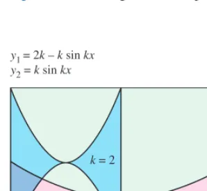
A Family of Butterflies

For each positive integer

k

, let

A

denote the area of the butterfly-shaped region

en-closed between the graphs of

y

k

sin

k x

and

y

2

k

k

sin

kx

on the interval

0,

p

k

. The regions for

k

1 and

k

2 are shown in Figure 7.7.

1.

Find the areas of the two regions in Figure 7.7.

2.

Make a conjecture about the areas

A

for

k

3.

3.

Set up a definite integral that gives the area

A

.

Can you make a simple

u

-substitution that will transform this integral into the definite integral that

gives the area

A

?

4.

What is lim

A

?

5.

If

P

denotes the perimeter of the

k

th butterfly-shaped region, what is

lim

P

? ( You can answer this question without an explicit formula for

P

.)

EXPLORATION 1

[0, ] by [0, 4] k = 2 y₁ = 2k – k sin kx y₂ = k sin kx

k = 1

Figure 7.7 Two members of the family

of butterfly-shaped regions described in Exploration 1.

Area Enclosed by Intersecting Curves

When a region is enclosed by intersecting curves, the intersection points give the limits of

integration.

EXAMPLE 2

Area of an Enclosed Region

Find the area of the region enclosed by the parabola

y

2

x

_{and the line}

_y

_x.

SOLUTION

We graph the curves to view the region ( Figure 7.8).

The limits of integration are found by solving the equation

2

x

_x

either algebraically or by calculator. The solutions are

x

1 and

x

2.

continued

y₁ = 2 – x2 y₂= – x

Since the parabola lies above the line on

1, 2

, the area integrand is 2

x

_x

_.

A

2

1

2

x

_x

_dx

[

2

x

x

3

3

x

₂

]

2

1

9

2

units squared

Now try Exercise 5.

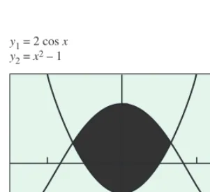
EXAMPLE 3

Using a Calculator

Find the area of the region enclosed by the graphs of

y

2 cos

x

and

y

x

_1.

SOLUTION

The region is shown in Figure 7.9.

Using a calculator, we solve the equation

2 cos

x

x

₁

to find the

x

-coordinates of the points where the curves intersect. These are the limits of

integration. The solutions are

x

1.265423706. We store the negative value as

A

and

the positive value as

B.

The area is

NINT

2 cos

x

x

₁

_,

_x

_,

_A

_,

_B

_4.994907788.

This is the final calculation, so we are now free to round. The area is about 4.99.

Now try Exercise 7.

Boundaries with Changing Functions

If a boundary of a region is defined by more than one function, we can partition the region

into subregions that correspond to the function changes and proceed as usual.

EXAMPLE 4

Finding Area Using Subregions

Find the area of the region

R

in the first quadrant that is bounded above by

y

x

and

below by the

x

- axis and the line

y

x

2.

SOLUTION

The region is shown in Figure 7.10.

y₁ = 2 cos x y2 = x2 – 1

x y

0 2

2

(4, 2)

y x 2

y 0 4

1

y ⎯√⎯x 2

B

A

Area ⌠⎮ √⎯⎯x x 2 dx

⌡

4 ⎡

⎣ ⎡⎣

Area ⌠⎮ √⎯⎯x dx

⌡

2

0

Figure 7.9 The region in Example 3.

Finding Intersections by Calculator

The coordinates of the points of inter-section of two curves are sometimes needed for other calculations. To take advantage of the accuracy provided by calculators, use them to solve for the values and storethe ones you want.

While it appears that no single integral can give the area of

R

(the bottom boundary is

defined by two different curves), we can split the region at

x

2 into two regions

A

and

B.

The area of

R

can be found as the sum of the areas of

A

and

B.

Area of

R

2

0

x

dx

4

2

x

x

2

dx

area of A area of B

2

3

x

32

]

0

[

2

3

x

32

x

2

2

2

x

]

4

2

1

3

0

units squared

Now try Exercise 9.

Integrating with Respect to

y

Sometimes the boundaries of a region are more easily described by functions of

y

than by

functions of

x.

We can use approximating rectangles that are horizontal rather than vertical

and the resulting basic formula has

y

in place of

x.

x

A =

∫

c

y

c

0

For regions like these

use this formula x_⫽ f(y) d

x y

c

0 d

x y

c 0 d

x_⫽ g(y)

x_⫽ f(y)

x_⫽ g(y)

x⫽ f(y) x_⫽ g(y)

EXAMPLE 5

Integrating with Respect to

y

Find the area of the region in Example 4 by integrating with respect to

y.

SOLUTION

We remarked in solving Example 4 that “it appears that no single integral can give the

area of

R,

” but notice how appearances change when we think of our rectangles being

summed over

y.

The interval of integration is

0, 2

, and the rectangles run between

the same two curves on the entire interval. There is no need to split the region

( Figure 7.11).

We need to solve for

x

in terms of

y

in both equations:

y

x

2

becomes

x

y

2,

y

x

becomes

x

y

_,

_y

_0.

continued

y

0 1

2 4

2

y 0

x y 2 x y2 (4, 2)

y (g(y), y)

(f(y), y)

f(y) g(y)

We must still be careful to subtract the lower number from the higher number when

form-ing the integrand. In this case, the higher numbers are the higher

x

-values, which are on

the line

x

y

2 because the line lies to the

right

of the parabola. So,

Area of

R

2

0

y

2

y

_dy

[

y

2

2

2

y

y

3

3

]

2

0

1

3

0

units squared.

Now try Exercise 11.

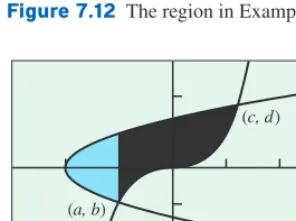
EXAMPLE 6

Making the Choice

Find the area of the region enclosed by the graphs of

y

x

_and

_x

_y

_2.

SOLUTION

We can produce a graph of the region on a calculator by graphing the three curves

y

x

_,

_y

_x

₂

_{, and}

_y

_x

₂

_{( Figure 7.12).}

This conveniently gives us all of our bounding curves as functions of

x.

If we integrate

in terms of

x

, however, we need to split the region at

x

a

( Figure 7.13).

On the other hand, we can integrate from

y

b

to

y

d

and handle the entire region

at once. We solve the cubic for

x

in terms of

y:

y

x

_becomes

_x

_y

_.

To find the limits of integration, we solve

y

_y

_{2. It is easy to see that the}

lower limit is

b

1, but a calculator is needed to find that the upper limit

d

1.793003715. We store this value as D.

The cubic lies to the right of the parabola, so

Area

NINT

y

_y

₂

_,

_y

_,

_{1, D}

_4.214939673.

The area is about 4.21.

Saving Time with Geometry Formulas

Here is yet another way to handle Example 4.

EXAMPLE 7

Using Geometry

Find the area of the region in Example 4 by subtracting the area of the triangular region

from the area under the square root curve.

SOLUTION

Figure 7.14 illustrates the strategy, which enables us to integrate with respect to

x

with-out splitting the region.

Area

4

0

x

dx

1

2

2

2

2

3

x

32

]

0

2

1

3

0

units squared

Now try Exercise 35.

The moral behind Examples 4, 5, and 7 is that you often have options for finding the

area of a region, some of which may be easier than others. You can integrate with respect to

x

or with respect to

y

, you can partition the region into subregions, and sometimes you can

even use traditional geometry formulas. Sketch the region first and take a moment to

deter-mine the best way to proceed.

[–3, 3] by [–3, 3] y₁ = x3_{, y}

2 = √x + 2, y3 = – √x + 2

(a, b)

(c, d)

Figure 7.12 The region in Example 6.

Figure 7.13 If we integrate with respect to xin Example 6, we must split the region at xa.

[–3, 3] by [–3, 3] (c, d)

(a, b)

x y

0 1

2

2 4 2

y 0

y x 2 2

Area 2 (4, 2)

y √⎯x

Figure 7.14 The area of the blue region is the area under the parabola y x

Quick Review 7.2

(For help, go to Sections 1.2 and 5.1.)

In Exercises 1–5, find the area between the x-axis and the graph of the given function over the given interval.

1. ysin x over 0,p 2

2. ye2x _{over 0, 1} 1

2(e21) 3.195

3. ysec2_{x over p}

In Exercises 6–10, find the x- and y-coordinates of all points where the graphs of the given functions intersect. If the curves never intersect, write “NI.”

6. yx2_{4x and yx6 (6, 12); (1, 5)} 7. yex _{and yx1 (0, 1)}

8. yx2_{px and ysinx (0, 0); (p, 0)} 9. y

x2 2

x

1

and yx3 _{(1,1); (0, 0); (1, 1)} 10. ysinx and yx3

Section 7.2 Exercises

In Exercises 1–6, find the area of the shaded region analytically.

1. p/2

2. 4p/3

3. 1/12

x y

1

0 1

(1, 1) x y3

x y2 t y

_– 3 1

– 4 0 2

y sec1_– 2 _t 2

_– 3 –

y 4 sin2 _{t –}

2

x y

y 1

0

y cos2_x 1

4. 4/3

5. 128/15

6. y 22/15

x 0

y x2 1

1

– 2 –1

y – 2x4

x y

y 2x2

2 (2, 8) 8

1 – 2

(– 2, 8)

y x4 2x2

–1

NOT TO SCALE

–1

1 x

y

0

1 _{x 12y}2 _12y3

x 2y2 2y